Current State
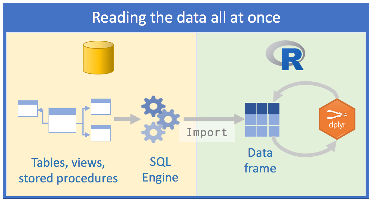
Using databases is unavoidable for those who analyze data as part of their jobs. As R developers, our first instinct may be to approach databases the same way we do regular files. We may attempt to read the data either all at once or as few times as possible. The aim is to reduce the number of times we go back to the data ‘well’, so our queries extract as much data as possible. After that, we spend cycles analyzing the data in memory. Here is what this model looks like:

Because the volume of data is significant with this approach, we usually attempt to come up with strategies to minimize the resources and time it takes to analyze the data. We may try to retrieve all rows of a few columns, or a few rows of several of columns. Another tactic is to save the query results into individual files for later analysis.
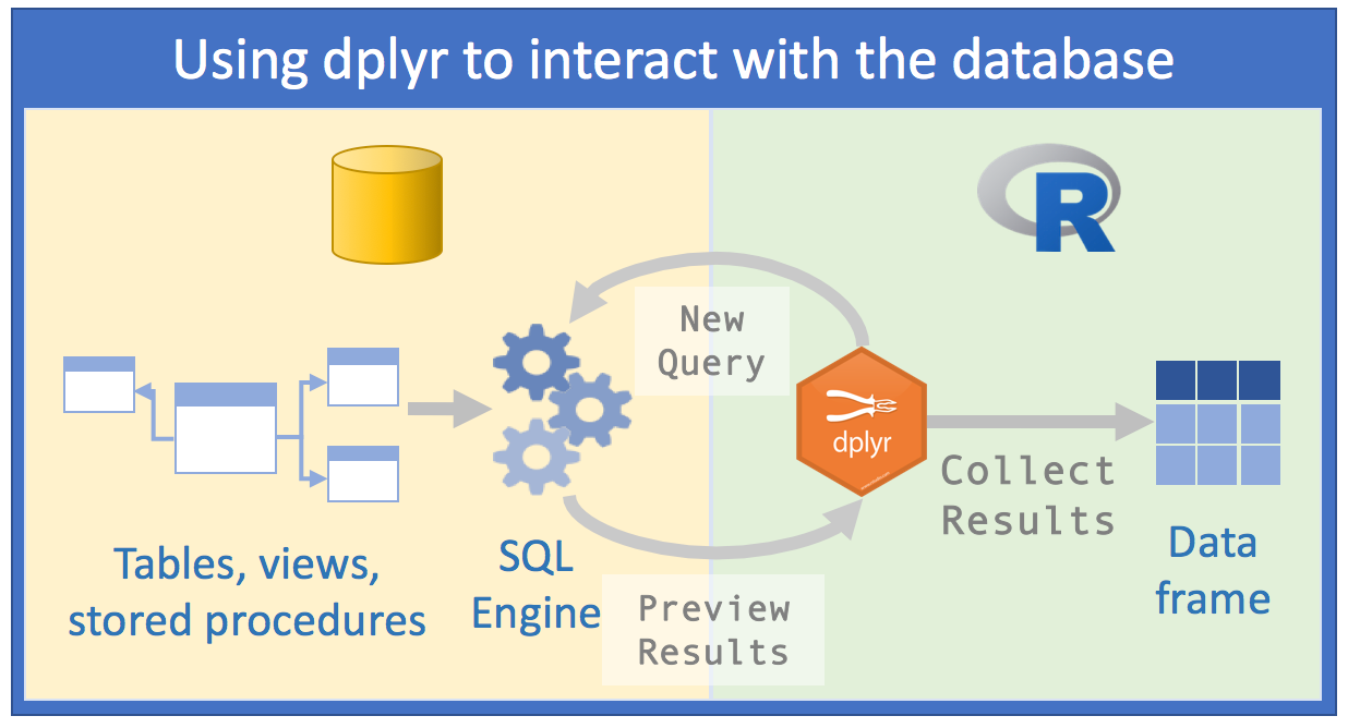
An improvement to the current approach would be to use the database’s SQL Engine to perform as much of the data exploration as possible. An enterprise-grade SQL server will have more power, and will be better tuned, to execute transformations of large amounts of data. Our goal would then be to bring into R a more targeted data set that will be used for visualization and modeling.
This improvement comes at a cost: we will need to know how to write SQL queries, and will have to switch between both languages. We may also end up using an external querying tool that is able to provide a list of tables and inline SQL code helpers. Of course, this involves switching between tools. On a personal note, I used to switch from R to Microsoft SQL Management Studio. After I that, I would bring the finalized query back into my code in R.
A better way

The dplyr package simplifies data transformation. It provides a consistent set of functions, called verbs, that can be used in succession and interchangeably to gain understanding of the data iteratively. The first time I re-wrote R code using dplyr, the new script was at least half as long and much easier to understand.
Another nice thing about dplyr is that it can interact with databases directly. It accomplishes this by translating the dplyr verbs into SQL queries. This incredibly convenient feature allows us to ‘speak’ directly with the database from R, thus resolving the issues brought up in the previous section:
Run data exploration over all of the data - Instead of coming up with a plan to decide what data to import, we can focus on analyzing the data inside the database, which in turn should yield faster insights.
Use the SQL Engine to run the data transformations - We are, in effect, pushing the computation to the database because
dplyris sending SQL queries to the database.Collect a targeted dataset - After become familiar with the data and choosing the data points that will either be shared or modeled, a final query can then be used to bring back only that data into memory in R.
All your code is in R! - Because we are using
dplyrto communicate with the database, there is no need to change language, or tools, to perform the data exploration.
Example
There are three things that we will need to get started:
A database we can access
A database driver installed in either our workstation or RStudio Server
All of the required packages installed in R
In this section, we will demonstrate how to access a Microsoft SQL Server database from a workstation that is running on Microsoft Windows.
Database Driver
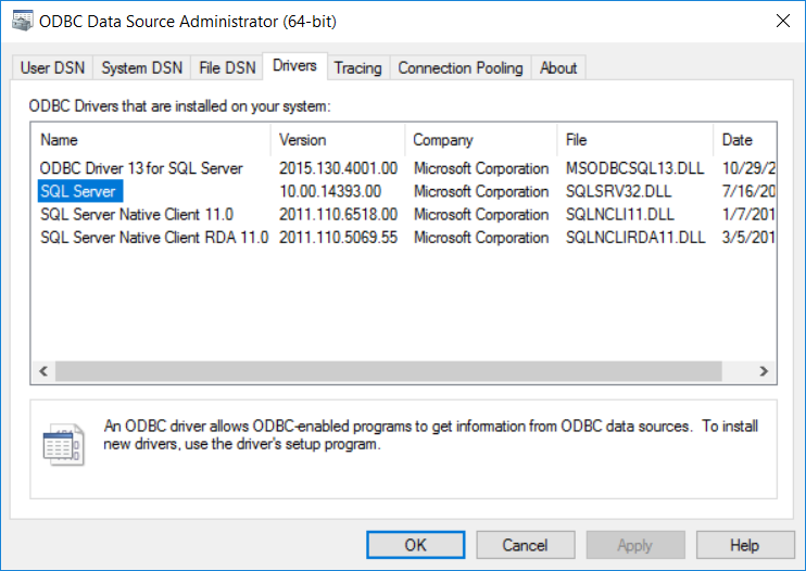
A database driver is a program that allows the workstation and the database to communicate. In Microsoft Windows, the drivers that connect to MS SQL databases are installed by default. We need the name of the driver that will be used inside our code in R. The easiest way to do this is to open the ODBC Data Source Administrator. To find it in your, system please refer to this article: Check the ODBC SQL Server Driver Version (Windows) . Once the administrator program is open, click on the Drivers tab. In my laptop, these are the drivers available. I will use SQL Server for the Driver argument in my connection in R.

R packages
Besides dplyr, the following packages are required:
odbc- This is the interface between the database driver and RDBI- Standardizes the functions related to database operationsdbplyr- Enablesdplyrto interact with databases. It also contains the vendor-specific SQL translations.
The database accessibility feature is still being developed, so we will use the development versions of dbplyr and dplyr.
devtools::install_github("tidyverse/dplyr")
devtools::install_github("tidyverse/dbplyr")
devtools::install_github("rstats-db/odbc")
install.packages("DBI")
Connect to the database
We will use the dbConnect() function from the DBI package to connect to the database. The value for the Driver argument is the name we determined in the Database Driver section above.
library(DBI)

con <- dbConnect(odbc::odbc(),
                   Driver    = "SQL Server",
                   Server    = "localhost",
                   Database  = "airontime",
                   UID       = [My User ID],
                   PWD       = [My Password],
                   Port      = 1433)
A very useful function in DBI is dbListTables(), which retrieves the names of available tables.
dbListTables(con)[1] "airlines" "airport" "airports" "faithful" "flights" "iris"
Another useful function is the dbListFields, which returns a vector with all of the column names in a table.
dbListFields(con, "flights")[1] "year" "month" "day" "dep_time" "sched_dep_time" [6] "dep_delay" "arr_time" "sched_arr_time" "arr_delay" "carrier" [11] "flight" "tailnum" "origin" "dest" "air_time" [16] "distance" "hour" "minute" "time_hour"
Interacting with the data using dplyr
Using dplyr, we can easily preview a database. The tbl() command creates a reference to the table.
library(dplyr)
tbl(con, "flights")
Source: table<flights> [?? x 19]
Database: Microsoft SQL Server 12.00.4422[username@localhost/airontime]
year month day dep_time sched_dep_time dep_delay arr_time sched_arr_time arr_delay carrier flight tailnum origin dest
<int> <int> <int> <int> <int> <dbl> <int> <int> <dbl> <chr> <int> <chr> <chr> <chr>
1 2013 1 1 517 515 2 830 819 11 UA 1545 N14228 EWR IAH
2 2013 1 1 533 529 4 850 830 20 UA 1714 N24211 LGA IAH
3 2013 1 1 542 540 2 923 850 33 AA 1141 N619AA JFK MIA
4 2013 1 1 544 545 -1 1004 1022 -18 B6 725 N804JB JFK BQN
5 2013 1 1 554 600 -6 812 837 -25 DL 461 N668DN LGA ATL
6 2013 1 1 554 558 -4 740 728 12 UA 1696 N39463 EWR ORD
7 2013 1 1 555 600 -5 913 854 19 B6 507 N516JB EWR FLL
8 2013 1 1 557 600 -3 709 723 -14 EV 5708 N829AS LGA IAD
9 2013 1 1 557 600 -3 838 846 -8 B6 79 N593JB JFK MCO
10 2013 1 1 558 600 -2 753 745 8 AA 301 N3ALAA LGA ORD
# ... with more rows, and 5 more variables: air_time <dbl>, distance <dbl>, hour <dbl>, minute <dbl>, time_hour <dttm>
The tally() verb in dplyr returns the row count.
tally(tbl(con, "flights"))Source: lazy query [?? x 1]
Database: Microsoft SQL Server 12.00.4422[username@localhost/airontime]
n
<int>
1 336776
When used against a database, the previous function is converted to a SQL query that works with MS SQL Server. The show_query() function displays the translation.
show_query(tally(tbl(con, "flights")))<SQL> SELECT COUNT(*) AS "n" FROM "flights"
Bringing it all together
The last code sample shows how easy it is to find out what the top airlines are by number of flights. Additionally, we wish to see the names of the airlines and not their codes. The steps taken are:
Start with the
flightstable and join it to thecarriertable to obtain the airline nameGroup the data by the airline
nameTally the total rows by airline
nameOrder the data by the resulting tallies in a descending order
All of these steps are translated into a SQL statement and processed inside the database. We do not need to import the tables into R memory at any time, we just use dplyr to get the results quickly.
tbl(con, "flights") %>%
  left_join(tbl(con, "airlines"), by = "carrier") %>%
  group_by(name) %>%
  tally %>%
  arrange(desc(n))
Source: lazy query [?? x 2]
Database: Microsoft SQL Server 12.00.4422[username@localhost/airontime]
Ordered by: desc(n)
# S3: tbl_dbi
name n
<chr> <int>
1 United Air Lines Inc. 58665
2 JetBlue Airways 54635
3 ExpressJet Airlines Inc. 54173
4 Delta Air Lines Inc. 48110
5 American Airlines Inc. 32729
6 Envoy Air 26397
7 US Airways Inc. 20536
8 Endeavor Air Inc. 18460
9 Southwest Airlines Co. 12275
10 Virgin America 5162
# ... with more rowsAdditional Resources
Here are links that will provide a deeper look into their respective subjects:
R for Data Science - An online book that covers how to use
dplyrand other like packages that together are called thetidyverse.
Conclusion
When we have only one method available to us, it is sometimes hard to see its inherent flaws. The method does what we need, so we do our best to overcome its shortfalls.
Our hope is that highlighting the issues related to importing large amounts of data into R, and the advantages of using dplyr to interact with databases, will be the encouragement needed to learn more about dplyr and to give it a try.
We plan to continue writing about the subject of databases using R in future posts. We will cover different aspects and techniques to get the most out of working with these two great technologies.
You may leave a comment below or discuss the post in the forum community.rstudio.com.