Introduction
Dynamic systems are usually represented by a model before they can be analyzed computationally. These dynamic systems are systems that change, evolve or have their states altered or varied with time based on a set of defined rules. Dynamic systems could be mechanical, electrical, electronic, biological, sociological, and so on. Many such systems are usually defined by a set rules that are represented as a set of nonlinear differential equations. A generic first-order differential form is as shown below: \[ \frac{dx}{dt} = f ( x(t), u(t), t ) ........... (1) \]
where x(t) is the state vector representing the configuration (or state) of the system at the time, t, u(t) represents the external control input at time, t, and f is a function that gives the rate of change of the state vector for a specific input, state and time.
The system of (1) could be said to be time invariant if we assume that f does not explicitly depend on time. This implies that the relation of (1) becomes:
\[ \frac{dx}{dt} = f (x, u) ........... (2) \]
For such time-invariant systems, the control input may remain time-variant, but the coefficients of the function f are constant since the underlying physical laws themselves are not usually time-dependent. Over a sufficiently small operating range, the dynamics of most systems are approximately linear, and the following relation entails a linear time-invariant (LTI) system:
\[ \frac{dx}{dt} = Ax + Bu ........... (3) \]
Several engineering challenges till today are being solved using LTI techniques, while most results obtained from control theory are based on the described assumptions associated with LTI systems.
Laplace Transform
For those systems that are described by differential equations, it is possible to convert the system’s time-domain model into a frequency-domain (s-domain) representation. Two striking benefits for doing this are:
- the differential equations that define the system are transformed into algebraic equations, which are often easier to analyze
- The frequency response of the system can be obtained
This frequency-domain output / input representation is called the transfer function. Many control system models are available in transfer function representation, and this model is mostly used in the block diagram representation of control systems.
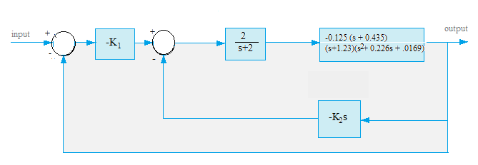
Figure 1 shows the block diagram for the pitch-control system of an Unmanned Free Swimming Submersible (UFSS) vehicle. This system and its block diagram shall be detailed in the Case Study section of this article.
Transfer Function Expressions
A transfer function expression is an algebraic expression in the frequency-domain. It is usually the ratio of the output to the input of a control system. Evaluating such expressions while retaining their mathematical form (as in symbolic mathematics) should be possible using a scientific computing language. An example of such expression is shown below:
\[ G(s) = \frac{Output}{Input} = \frac{s^2 + 3s + 4}{2s^3 + 4s^2 + 5s + 1} \]
Models of physical systems often appear as transfer functions with the coefficients of state as electrical, mechanical, chemical, or other physical quantities. Users would find it convenient to simply input these transfer functions as-is into a computer, and quickly analyze the system.
In the following mechanical example of a mass-spring-damper system of [1], the transfer function contains symbols m, b and k, which represent mass, damping constant, and spring constant variables respectively, as shown below:
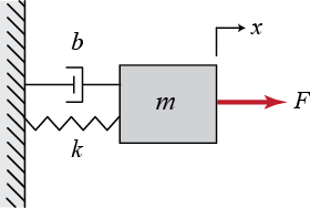 Figure 2: Mass-Spring-Damper diagram \[
\frac{X(s)}{F(s)} = \frac{1}{ms^2+bs+k}
\]
where m = 1; k = 1; b = 0.2
In this Google Summer of Code (GSoC) 2017 project, we have tried to include such capability within the control library, making it possible to create a transfer function model from the evaluation of a rational expression (the transfer function). A function named TF() was created to accept transfer function expressions, and return a transfer function model after evaluation. Therefore, to create this mass-spring-damper model within R, use the control library as shown in the snippet below:
 m <- 1;  k <- 1;  b <- 0.2
TF("1/(m*s^2 + b *s + k)")
##
## y1:
## 1
## - - - - - - - - - - -
## s^2 + 0.2 s + 1
##
##
## Transfer Function: Continuous time model.
Electric Motor Example
Consider the following example from a University of Michigan course page on Control Systems using MATLAB – an example of an electric motor [2]
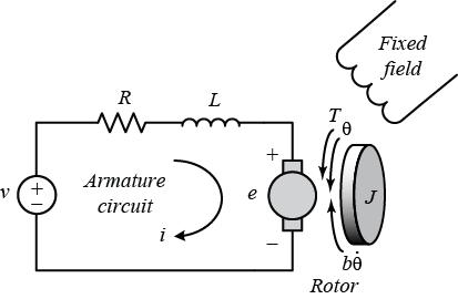 Figure 3: showing electric motor physical model [2]
Wikipedia: A DC motor is any class of rotary electric machines that converts direct current electrical energy into mechanical energy. It can provide translational motion when coupled with wheel, drums and cables. DC motors are used in propulsion of electric vehicles, elevator and hoists, or in drives for steel rolling mills. Several applications are: air compressors, vacuum cleaner, hair drier, sewing machine, and even toys or any system that requires variable speed.
The physical parameters for this example are [3]:
Moment of inertia of the rotor, J = 3.2284E-6 kg.m^2
Motor viscous friction constant, b = 3.5077E-6 N.m.s
Electromotive force constant, Ke = 0.0274 V/rad/sec
Motor torque constant, Kt = 0.0274 N.m/Amp
Electric resistance, R = 4 Ohm
Electric inductance, L = 2.75E-6 H
where, Kt = Ke = K
The input of the system is the voltage source (V) applied to the motor’s armature, while the output is the rotational speed of the shaft.
Open-Loop Response of the electric motor
The open-loop transfer function for the DC motor described above in the s-domain is:
\[ P(s) = \frac{K}{(s(Js + b)(Ls + R) + K^2)} \]
The step function is usually used to analyze the system’s step response, so it is applied here to analyze the open-loop response of the system. Using the control library, this model in the s-domain could be created and analyzed in R as follows:
 J <- 3.2284E-6;
b <- 3.5077E-6;
K <- 0.0274;
R <- 4;
L <- 2.75E-6;
P_motor <- TF("K/(s*((J*s + b)*(L*s + R) + K^2))")
time <- seq(0,0.2,0.001)
stepplot(P_motor, t = time)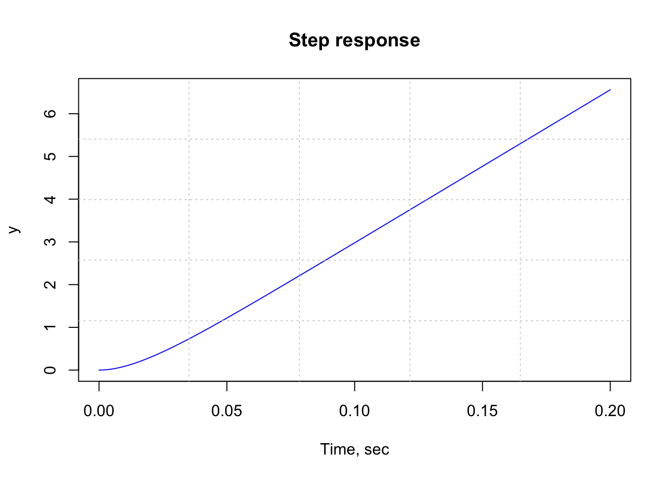
Figure 1: Figure 4: Electric Motor Open-loop Step Response
From the above plot showing the system’s step response, it is clear that when a step input (of 1 volt) is applied to the system, the electric motor’s position grows unbounded - system instability.
The stability of the system can also be determined from the poles of the transfer function using the pole function:
pole(P_motor)## [,1]
## [1,] 0.000000e+00
## [2,] -1.454487e+06
## [3,] -5.922604e+01As shown above, one of the poles of the open-loop transfer function is on the imaginary axis while the other two poles are in the left half of the complex s-plane. A pole on the imaginary axis indicates that the free response of the system will not only grow unbounded, but also will not decay to zero [3].
Closed-Loop Response of the electric motor
We can add feedback the motor model with a controller set to 1, and then investigate the system’s closed-loop step response for stability. This can be obtained using the following R commands:
P_motor2 <- feedback(P_motor, 1)
print(P_motor2)
##
## y1:
## 0.0274
## - - - - - - - - - - - - - - - - - - - - - - - - - - - - - - - - -
## 8.8781e-12 s^3 + 1.291361e-05 s^2 + 0.0007647908 s + 0.0274
##
##
## Transfer Function: Continuous time model# OR
P_motor2 <- cloop(P_motor, -1)
print(P_motor2)##
## y1:
## 0.0274
## - - - - - - - - - - - - - - - - - - - - - - - - - - - - - - - - -
## 8.8781e-12 s^3 + 1.291361e-05 s^2 + 0.0007647908 s + 0.0274
##
##
## Transfer Function: Continuous time modelstepplot(P_motor2, t = time)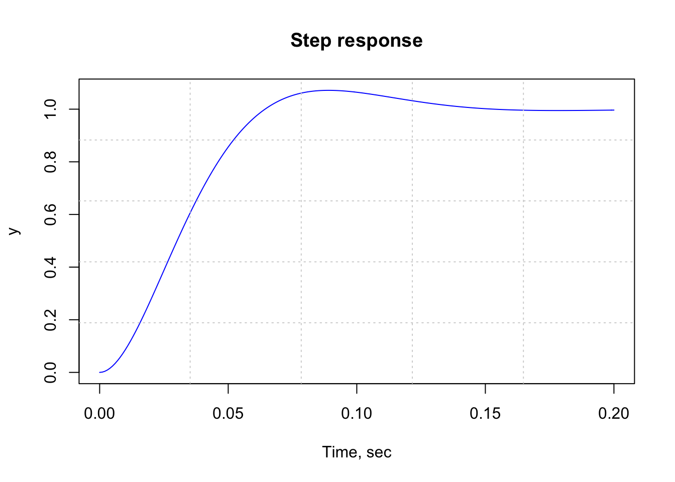
Figure 2: Figure 5: Electric Motor Closed-loop Step Response
The above closed-loop step response shows that the addition of feedback has stabilized the system.
The damping and natural frequencies associated with the poles of this closed-loop system could be obtained using the following damp function:
damp(P_motor2)##
## Eigenvalue Damping Freq. (rad/s) Freq. (Hz).
## ---------- ------- ------------- -----------
## -29.61 + 35.28j 0.64 46.06 0.46
## -29.61 - 35.28j 0.64 46.06 0.46
## -1454487.32 + 0.00j 1.00 1454487.32 0.00## $omega
## [,1]
## [1,] 4.606386e+01
## [2,] 4.606386e+01
## [3,] 1.454487e+06
##
## $zeta
## [1] 0.642853 0.642853 1.000000Furthermore, using the TF() function, transfer function models could be summed, subtracted, multiplied, and divided. This is exemplified in the following section.
System Interconnections
In many cases, systems or subsystems have to be interconnected to obtain a particular controlled or regulated activity. Interconnecting models of components allows you to easily construct large control system models.
Analyzing systems that are modeled in a block diagram should be easily done using a scientific computing tool like R. The time response or frequency response of a system (such as shown in Figure 1), can be obtained after the block diagram is simplified. Simplification means that the several components (blocks described by different transfer functions) that make up the complete system have to be algebraically reduced to one transfer function to represent the system. This mathematical reduction is done based on the rules of control theory.

Figure 6: Block Diagram Interconnection
For an example, Figure 6 shows the interconnection of dynamic system models of a plant P(s), a controller C(s), sensor dynamics S(s), and a filter F(s). To analyze the system requires constructing a single (equivalent) model that represents the entire closed-loop control system.
In the second coding phase of the GSoC 2017, the following model interconnection functions have been produced as shown in Figure 7 below:
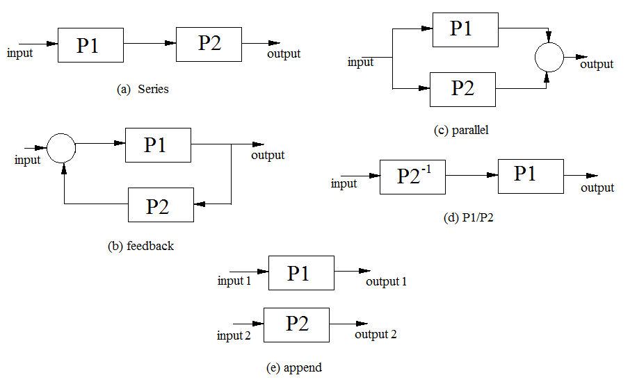
Figure 7: System Model Interconnections
Append Connection using the append function
A number of systems, whether in transfer-function, state-space or zero-pole model, could be appended into one state-space model using the append function. The block diagram arrangement is found in Figure 7 (e).
The syntax is: append(sys1, sys2, …, sysN). The resulting model is in state-space form.
For example:
 sys1 <- ss(1,2,3,4)
 sys2 <- ss(2,3,4,5)
 sys3 <- ss(6,7,8,9)
 sys4 <- tf(1, c(1,2,5))
 append(sys1, sys2, sys3)
 append(sys1, sys2, sys4, sys3)
.
Series Connection using the series function
This function connects two systems in series, in transfer-function, state-space or zero-pole model, into one model. The block diagram arrangement is found in Figure 7 (a).
Syntax: series(sys1, sys2)
Arithmetically, this could be achieved using the TF() function in the following manner:
TF(“sys1*sys2”)
For now, TF(“sys1*sys2”) is only possible when sys1 and sys2 are transfer-function models
.
Parallel Connection using the parallel function
The parallel function connects two systems in parallel, in transfer-function, state-space or zero-pole model, into one model. The block diagram arrangement is found in Figure 7 (c).
Syntax: parallel(sys1, sys2)
Arithmetically, this could be achieved using the TF() function in the following manner:
TF(“sys1 + sys2”)
For now, TF(“sys1+ sys2”) is only possible when sys1 and sys2 are transfer-function models
.
Feedback Connection using the feedback function
This function sets up a closed-loop transfer function from output to input based on the standard configuration shown in Figure 7 (b).
Syntax: feedback(sys1, sys2)
Arithmetically, this could be achieved using the TF() function in the following manner:
TF(“sys1 / (1 + sys2*sys1)”), but this is not recommended in terms of accuracy. feedback(sys1, sys2) is preferred.
.
General block diagram building using connect function
Using the connect function, more complicated (especially multiple-input multiple-output (MIMO) ) block diagrams could be set up. For this case, all systems that are to be connected are first appended, then connected using their inputs and outputs.
Syntax: connect(append(sys1, sys2, sys3), connections, inputs, outputs)
.
Case Study – Unmanned Free Swimming Submersible (UFSS) Vehicle
The Unmanned Free-Swimming Submersible (UFSS) vehicle was one of the first autonomous underwater vehicles (AUVs). It was developed in the late 1970s as a test vehicle to demonstrate the potential of autonomous vehicles over long distances, and to study laminar flow [5]. A picture showing an Unmanned Free-Swimming Submersible (UFSS) vehicle is shown in Figure 8 below.
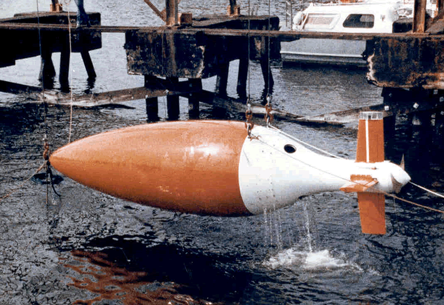
Figure 8: Unmanned Free Swimming Submersible Vehicle (UFSS). Source: [5]
Nise [4] relates the following concerning the UFSS:
The depth of the vehicle is controlled as follows. During forward motion, an elevator surface on the vehicle is deflected by a selected amount. This deflection causes the vehicle to rotate about the pitch axis. The pitch of the vehicle creates a vertical force that causes the vehicle to submerge or rise.
A detailed block diagram for the pitch control system is shown in Figure 9 below.
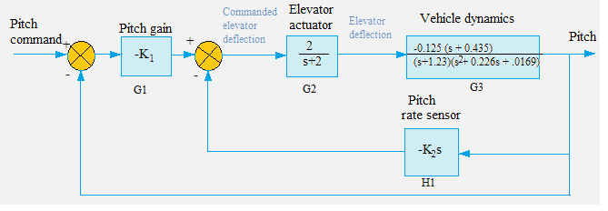
Figure 9: Block diagram for the pitch control system of UFSS
Rationale:
The subsystems of the UFSS vehicle are developed independently, and studied using computer simulation before integration into the vehicle [5]. Thus, for this reason, we are examining the pitch control system independently.
For this case study, we shall use the developing control library in R to:
- Obtain the closed-loop UFSS pitch control system by block diagram reduction of the system in Figure 9 above, using
series,parallelandfeedback. - Obtain the step response of the pitch control system simplified by
series,parallelandfeedback - Obtain the closed-loop UFSS pitch control system by block diagram reduction of the system in Figure 9 above, using the algebraic operations provided by
TF(). - Obtain the step response of the pitch control system from the method of algebraic operations.
Solution using series, parallel and feedback
K1 <- 1
K2  <- 1
G1 <- tf(-K1,1)
G2 <- tf(c(0,2), c(1,2))

numg3 <- -0.125*c(1, 0.435)
deng3 <- pracma::polymul(c(1, 1.23), c(1, 0.226, 0.0169))
G3 <- tf(numg3, deng3)

H1 <- tf(c(-K2, 0), c(0, 1))

G4 <- series(G2, G3)
G5 <- feedback(G4, H1)
Ge <- series(G1, G5)
T1 <- feedback(Ge, 1)
stepplot(T1, t = seq(0,40,0.1))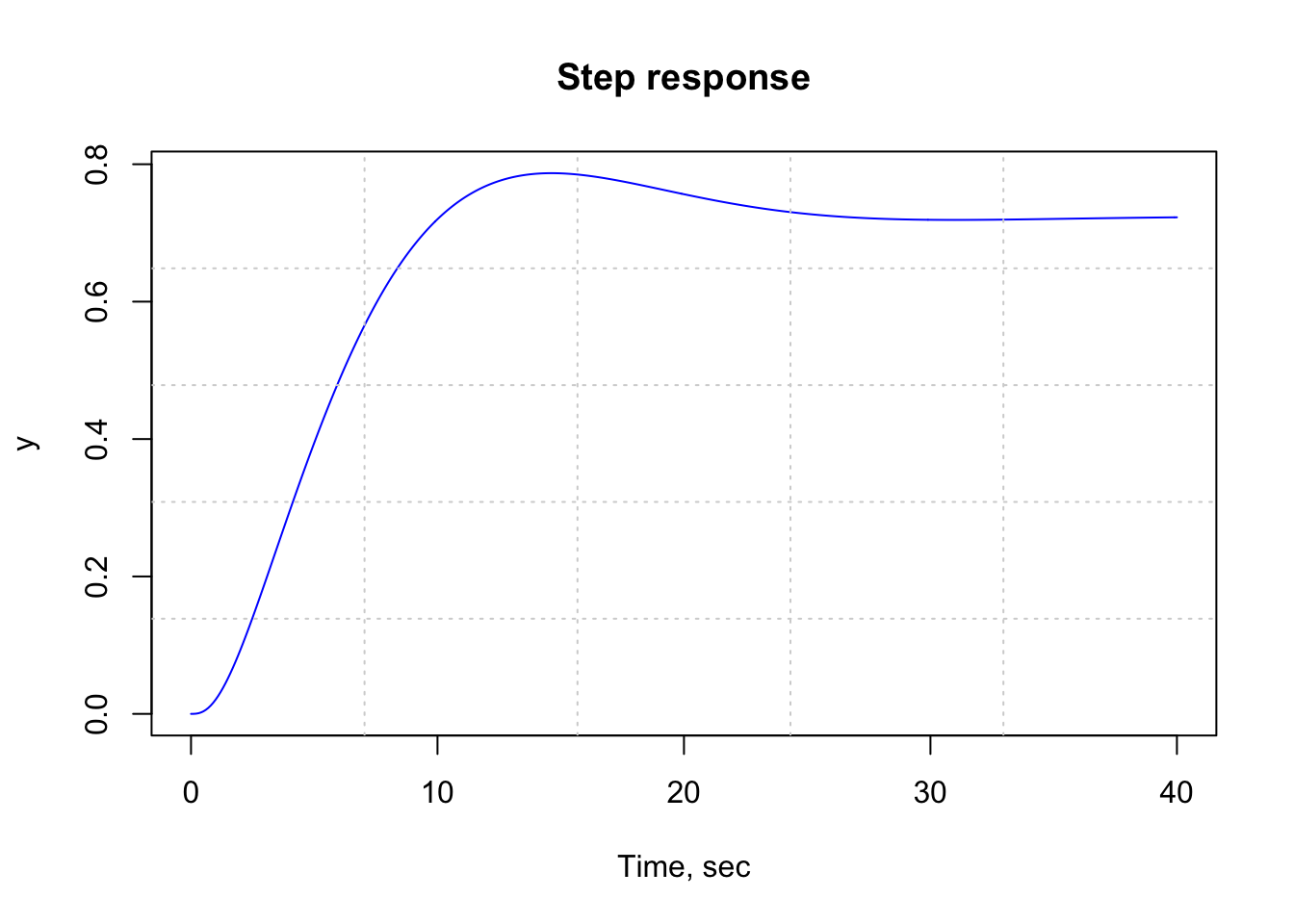
Figure 3: Figure 10: R plot showing UFSS vehicle system response - Block diagram reduction by series, parallel and feedback
Solution via algebraic operations
G4 <- TF("G3*G2")
G5 <- TF("G4/(1+ G4*H1)")
Ge <- TF("G5*G1")
T2 <- TF("Ge/(1+Ge)")
stepplot(T2, t = seq(0,40,0.1))
Figure 4: Figure 11: R plot showing UFSS vehicle system response - Block diagram reduction by Algebraic Operations
Clearly, the step responses (Figure 10 and Figure 11) of the pitch control system using the two methods are identical to each other - a justification to the framework of the control systems toolbox.
Feedback
Interested users are welcome to install the development version of this package using devtools::install_github("benubah/control"), and feel free to get in touch for any related issues.
.
Conclusion
In this article, we have discussed on our progress with the Control Systems Toolbox in R as a GSoC 2017 project. We have highlighted the use of this toolbox to carry out the following tasks:
- Create Transfer function models by evaluating transfer function expressions in the s-domain
- Obtain the poles and their associated damping and natural frequencies of a system
- Open-loop and closed-loop responses
- System Model Interconnections using series, parallel and feedback and algebraic functions in the UFSS vehicle case study.
Other functions that have been developed in this GSoC phase are: givens_rot, ordschur, care, ctrb, acker, place.
You may want to read about what was achieved in the first GSoC coding phase here.
References
http://ctms.engin.umich.edu/CTMS/index.php?example=Introduction§ion=SystemModeling
http://ctms.engin.umich.edu/CTMS/index.php?example=MotorSpeed§ion=SystemModeling
http://ctms.engin.umich.edu/CTMS/index.php?example=MotorPosition§ion=SystemAnalysis
Norman, S. Nise, Control Systems Engineering, 6th. Ed, 2011.
You may leave a comment below or discuss the post in the forum community.rstudio.com.