In our previous portfolio volatility work, we covered how to import stock prices, convert to returns and set weights, calculate portfolio volatility, and calculate rolling portfolio volatility.
Now we want to break that total portfolio volatility into its constituent parts and investigate how each asset contributes to the volatility. Why might we want to do that?
For our own risk management purposes, we might want to ensure that our risk isn’t too concentrated in one asset. Not only might this lead to a less-diversified portfolio than we thought we had, but it also might indicate that our initial assumptions about a particular asset were wrong - or, at least, they have become less right as the asset has changed over time.
Similarly, if this portfolio is governed by a mandate from, say, an institutional client, that client might have a preference or even a rule that no asset or sector can rise above a certain threshold of risk contribution. That institutional client might require a report like this from each of their outsourced managers, so they can sum the constituents.
With that motivation in mind, let’s get prices, returns, and set weights for five ETFs.
library(timetk)
library(tidyverse)
library(tidyquant)
library(highcharter)


symbols <- c("SPY","IJS","EFA","EEM","AGG")

prices <-
  getSymbols(symbols, src = 'google', from = "2005-01-01",
             auto.assign = TRUE, warnings = FALSE) %>%
  map(~Cl(get(.))) %>%
  reduce(merge) %>%
  `colnames<-`(symbols)

prices_monthly <- to.monthly(prices, indexAt = "first", OHLC = FALSE)

portfolioComponentReturns <- na.omit(Return.calculate(prices_monthly, method = "log"))

w = c(0.25, 0.20, 0.20, 0.25, 0.10)
We need to build the covariance matrix and calculate portfolio standard deviation.
covariance_matrix <- cov(portfolioComponentReturns)

# Square root of transpose of the weights cross prod covariance matrix returns
# cross prod weights gives portfolio standard deviation.
sd_portfolio <- sqrt(t(w) %*% covariance_matrix %*% w)
Let’s start to look at the individual components.
The percentage contribution of asset i is defined as:
(marginal contribution of asset i * weight of asset i) / portfolio standard deviation
To find the marginal contribution of each asset, take the cross-product of the weights vector and the covariance matrix divided by the portfolio standard deviation.
# Marginal contribution of each asset.
marginal_contribution <- w %*% covariance_matrix / sd_portfolio[1, 1]
Now multiply the marginal contribution of each asset by the weights vector to get total contribution. We can then sum the asset contributions and make sure it’s equal to the total portfolio standard deviation.
# Component contributions to risk are the weighted marginal contributions
component_contribution <- marginal_contribution * w

# This should equal total portfolio vol, or the object `sd_portfolio`
components_summed <- rowSums(component_contribution)
The summed components are 0.0448135 and the matrix calculation is 0.0448135.
To get to percentage contribution of each asset, we divide each asset’s contribution by the total portfolio standard deviation.
# To get the percentage contribution, divide component contribution by total sd.
component_percentages <- component_contribution / sd_portfolio[1, 1]
Let’s port this to a tibble for ease of presentation, and we’ll append by_hand to the object because we did the calculations step-by-step.
percentage_tibble_by_hand <-
  tibble(symbols, w, as.vector(component_percentages)) %>%
  rename(asset = symbols, 'portfolio weight' = w, 'risk contribution' = `as.vector(component_percentages)`)

percentage_tibble_by_hand
## # A tibble: 5 x 3
## asset `portfolio weight` `risk contribution`
## <chr> <dbl> <dbl>
## 1 SPY 0.25 0.213569366
## 2 IJS 0.20 0.213310709
## 3 EFA 0.20 0.220213245
## 4 EEM 0.25 0.349901018
## 5 AGG 0.10 0.003005661As you might have guessed, we used by_hand in the object name because we could have used a pre-built R function to do all this work.
The StdDev function from PerformanceAnalytics will run this same calculation if we pass in the weights and set portfolio_method = "component" (recall that if we set portfolio_method = "single", the function will return the total portfolio standard deviation, as we saw in our previous work).
Let’s confirm that the pre-built function returns the same results.
# Confirm component contribution to volality.
component_sd_pre_built <- StdDev(portfolioComponentReturns, weights = w,
                              portfolio_method = "component")
component_sd_pre_built
## $StdDev
## [,1]
## [1,] 0.04481354
##
## $contribution
## SPY IJS EFA EEM AGG
## 0.0095707991 0.0095592078 0.0098685349 0.0156803030 0.0001346943
##
## $pct_contrib_StdDev
## SPY IJS EFA EEM AGG
## 0.213569366 0.213310709 0.220213245 0.349901018 0.003005661That function returns a list, and one of the elements is $pct_contrib_StdDev, which is the percentage contribution of each asset. Let’s move it to a tibble for ease of presentation.
# Port to a tibble.
percentages_tibble_pre_built <-
  component_sd_pre_built$pct_contrib_StdDev %>%
  tk_tbl(preserve_row_names = FALSE) %>%
  mutate(asset = symbols) %>%
  rename('risk contribution' = data) %>%
  select(asset, everything(), -index)
Has our work checked out? Is percentages_tibble_pre_built showing the same result as component_percentages_tibble_by_hand?
Compare the two objects
percentages_tibble_pre_built## # A tibble: 5 x 2
## asset `risk contribution`
## <chr> <dbl>
## 1 SPY 0.213569366
## 2 IJS 0.213310709
## 3 EFA 0.220213245
## 4 EEM 0.349901018
## 5 AGG 0.003005661percentage_tibble_by_hand## # A tibble: 5 x 3
## asset `portfolio weight` `risk contribution`
## <chr> <dbl> <dbl>
## 1 SPY 0.25 0.213569366
## 2 IJS 0.20 0.213310709
## 3 EFA 0.20 0.220213245
## 4 EEM 0.25 0.349901018
## 5 AGG 0.10 0.003005661Huzzah - our findings seem to be consistent!
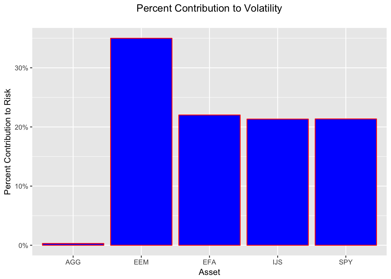
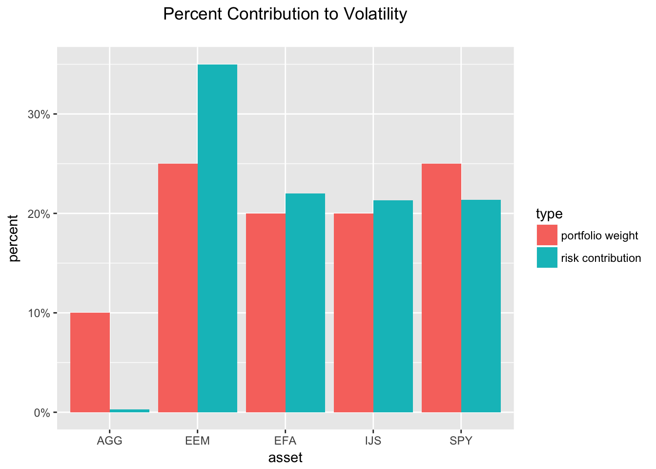
While we have the tibbles in front of us, notice that EEM has a 25% weight but contributes 35% to the volatility. That’s not necessarily a bad thing, but we should be aware of it.
Our substantive work is done, but let’s turn to ggplot for some visualization.
component_percent_plot <-
  ggplot(percentage_tibble_by_hand, aes(asset, `risk contribution`)) +
  geom_col(fill = 'blue', colour = 'red') +
  scale_y_continuous(labels = scales::percent) +
  ggtitle("Percent Contribution to Volatility",
          subtitle = "") +
  theme(plot.title = element_text(hjust = 0.5)) +
  theme(plot.subtitle = element_text(hjust = 0.5)) +
  xlab("Asset") +
  ylab("Percent Contribution to Risk")

component_percent_plot
How about a chart that compares weights to risk contribution? First we’ll need to gather our tibble to long format, then call ggplot.
# gather
percentage_tibble_by_hand_gather <-
  percentage_tibble_by_hand %>%
  gather(type, percent, -asset)

# built ggplot object
plot_compare_weight_contribution <-
  ggplot(percentage_tibble_by_hand_gather, aes(x = asset, y = percent, fill = type)) +
  geom_col(position = 'dodge') +
  scale_y_continuous(labels = scales::percent) +
  ggtitle("Percent Contribution to Volatility",
          subtitle = "") +
  theme(plot.title = element_text(hjust = 0.5)) +
  theme(plot.subtitle = element_text(hjust = 0.5))

plot_compare_weight_contribution
It looks like AGG, a bond fund, has done a good job as a volatility dampener. It has a 10% allocation but contributes almost zero to volatility. We’re ignoring returns for now.
The largest contributor to the portfolio volatility has been EEM, an emerging market ETF, but have a look at the EEM chart and note that it’s own absolute volatility has been quite low.
EEM_sd <- StdDev(portfolioComponentReturns$EEM)

EEM_sd_overtime <-
  round(rollapply(portfolioComponentReturns$EEM, 20, function(x) StdDev(x)), 4) * 100

highchart(type = "stock") %>%
  hc_title(text = "EEM Volatility") %>%
  hc_add_series(EEM_sd_overtime, name = "EEM Vol") %>%
  hc_yAxis(labels = list(format = "{value}%"), opposite = FALSE) %>%
  hc_navigator(enabled = FALSE) %>%
  hc_scrollbar(enabled = FALSE)
EEM has contributed 35% to portfolio volatility, but it hasn’t been very risky over this time period. It’s standard deviation has been 0.0671957. Yet, it is still the riskiest asset in our portfolio. Perhaps this is a safe portfolio? Or perhaps we are in a period of very low volatility (indeed, that is the case according to the VIX and actual realized volatility).
That’s all for today. See you next time.
You may leave a comment below or discuss the post in the forum community.rstudio.com.