Climate Change and Population Modeling in R

A recent paper in nature climate change: Less than 2°C warming by 2100 unlikely (Raftery et al. 2017), concludes that the goal of the Paris Agreement is unlikely to be met.

Although the conclusion is disheartening, the paper advances the science of climate modeling by developing a joint Bayesian hierarchical model for Gross Domestic Product per capita and carbon intensity. This ensemble of models, in turn, depends on the availability of probabilistic population projections developed by the BayesPop Project at the University of Washington and available on CRAN.

The linkage between CO₂ emissions and population modeling comes through the use of a version of the Kaya identity, which “expresses future emissions levels in a country as a product of three components: population, GDP per capita, and carbon intensity (CO₂ emissions per unit of GDP).”

The 3700 lines of R code that implement the models underlying the paper are available here on GitHub. Unless you work in this aspect of climate modeling, mastering this code seems likely to be a formidable task. A good first step, however, might be to work through the population models developed by BayesPop. These models comprise a series of R packages:

• bayesTFR implements a Bayesian hierarchical model to make projections of total fertility for all of the countries in the world.
  
• bayesLife implements a Bayesian Hierarchical model to make life expectancy projections for all the countries in the world is described here.
  
• bayesPop uses bayesTFR and bayesLife to generate population projections for all of the world’s countries.
  
• bayesDem provides graphical user interface for bayesTFR, bayesLife and bayesPop.
  
• wppExployer implements a shiny app for exploring the data in on the World Population Prospects This data is available in R packages wpp2017, wpp2015, wpp2012, and wpp2010,

The wppExployer shiny app is also available online.

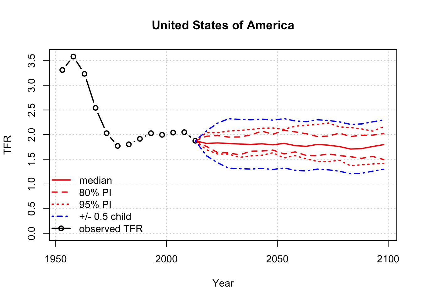
To give you a feel for how these models work, we use the bayesTFR package to estimate and plot fertility rates for the United States. (Note that, for brevity, the informative console output of the simulations in the code below have been suppressed.)

library(bayesTFR)
# This command produces output data, such as in the directory ex-data
sim.dir <- tempfile()
# Phase II MCMCs
m <- run.tfr.mcmc(nr.chains=1, iter=60, output.dir=sim.dir, seed=1, verbose=TRUE)

## Loading required package: wpp2017

## Warning: package 'wpp2017' was built under R version 3.4.2

# Phase III MCMCs (not included in the package)
m3 <- run.tfr3.mcmc(sim.dir=sim.dir, nr.chains=2, iter=100, thin=1, seed=1, verbose=TRUE)
# Prediction
pred <- tfr.predict(m, burnin=30, burnin3=50, verbose=TRUE)
summary(pred, country='United States of America')
unlink(sim.dir, recursive=TRUE)

tfr.trajectories.plot(pred,country="United States of America")

The transparent, reproducible work being done by Raftery and his collaborators, and the other members of the BayesPop Project, is a great gift to the R community. Anyone with an appetite for R code and the patience to learn something of Bayesian hierarchical models can gain some insight into one of the most important scientific problems of our day.