I have been searching for various ways to find information about R packages for some time now, but I only recently learned about the CRAN_package_db() function in the base tools package. If a colleague hadn’t pointed it out to me, I am sure I would never have found it on my own.
pdb <- tools:::CRAN_package_db() When invoked, this function goes out to the CRAN mirror specified by the environment variable R_CRAN_WEB and returns a data frame containing a whole lot of information about each package currently on CRAN. It is a treasure trove of meta data.
load(file="../../static/post/2018-02-26-Rickert-CRAN-metadata_files/pdbJan31.RDA")
class(pdb)
## [1] "data.frame"dim(pdb)## [1] 12123 65names(pdb)## [1] "Package" "Version"
## [3] "Priority" "Depends"
## [5] "Imports" "LinkingTo"
## [7] "Suggests" "Enhances"
## [9] "License" "License_is_FOSS"
## [11] "License_restricts_use" "OS_type"
## [13] "Archs" "MD5sum"
## [15] "NeedsCompilation" "Additional_repositories"
## [17] "Author" "Authors@R"
## [19] "Biarch" "BugReports"
## [21] "BuildKeepEmpty" "BuildManual"
## [23] "BuildResaveData" "BuildVignettes"
## [25] "Built" "ByteCompile"
## [27] "Classification/ACM" "Classification/ACM-2012"
## [29] "Classification/JEL" "Classification/MSC"
## [31] "Classification/MSC-2010" "Collate"
## [33] "Collate.unix" "Collate.windows"
## [35] "Contact" "Copyright"
## [37] "Date" "Description"
## [39] "Encoding" "KeepSource"
## [41] "Language" "LazyData"
## [43] "LazyDataCompression" "LazyLoad"
## [45] "MailingList" "Maintainer"
## [47] "Note" "Packaged"
## [49] "RdMacros" "SysDataCompression"
## [51] "SystemRequirements" "Title"
## [53] "Type" "URL"
## [55] "VignetteBuilder" "ZipData"
## [57] "Published" "Path"
## [59] "X-CRAN-Comment" "Reverse depends"
## [61] "Reverse imports" "Reverse linking to"
## [63] "Reverse suggests" "Reverse enhances"
## [65] "MD5sum"Working with the information returned may require a bit of data wrangling. In this post, I’ll show a cleaned-up (but far from elegant) version of some of the work I did to prepare for my rstudio::conf 2018 talk, What Makes a Great R Package?, as an example of working with the character data. I was interested in getting a sense of the collaboration that goes into writing a typical R package, along with a feel for how useful a package may be for other package developers. The proxy I chose for collaboration is the number of authors listed for each package. My proxy for usefulness to other package developers was the union of reverse depends and reverse imports.
The first thing I did was select a subset of the data frame to work on.
meta_data <- pdb[, c(1,4,5,17,60,61)]
names(meta_data) <- c("Package","Dep","Imp","Aut","RD","RI")
glimpse(meta_data)
## Observations: 12,123
## Variables: 6
## $ Package <chr> "A3", "abbyyR", "abc", "abc.data", "ABC.RAP", "ABCanal...
## $ Dep <chr> "R (>= 2.15.0), xtable, pbapply", "R (>= 3.2.0)", "R (...
## $ Imp <chr> NA, "httr, XML, curl, readr, plyr, progress", NA, NA, ...
## $ Aut <chr> "Scott Fortmann-Roe", "Gaurav Sood [aut, cre]", "Csill...
## $ RD <chr> NA, NA, "abctools, EasyABC", "abc", NA, NA, NA, NA, NA...
## $ RI <chr> NA, NA, "ecolottery", NA, NA, NA, NA, NA, NA, NA, NA, ...Note that in this post, I am using data from a file I pulled from CRAN just before my talk, but you should not have any trouble working with CRAN_package_db() to get an updated data set.
The next thing I did was to add two new variables to the data set: DepImp, the union of the dependent packages and imported packages, and RDRI, the union of the reverse depends and reverse imports packages.
library(stringr)
# A helper function to unlist and string split.
fcn <- function(x,y){
  x <- unlist(x) %>% strsplit(",")
  y <- unlist(y) %>% strsplit(",")
  z <- unlist(na.omit(union(x, y)))
}

meta_data <- mutate(meta_data,
                DepImp = mapply(fcn,Dep,Imp),
                RDRI = mapply(fcn,RD,RI))
Also, it turned out that the Authors field needed a bit of work in order to remove the qualification text like “[aut, cre]” and “[ctb, cph]” from the strings of authors.
# CLEAN THE AUTHOR'S FIELD
# Function to remove all text between two brackets
# http://bit.ly/2mE7TNJ
clean <- function(x){
  gsub("\\[[^]]*]", "",x)
}

# Function to remove line breaks
# http://bit.ly/2B0n4VS

clean2 <- function(x){
  gsub("[\r\n]", "", x)
}

# Clean Author's field
meta_data$Aut <- meta_data$Aut %>% map(clean) %>% map(clean2)
Once I had some clean text, I used a very messy preliminary version of the following code to obtain the count data I was looking for. Note that the derived features, DepImp and RDRI, need some pre-processing that is different from that which is required to extract counts from the other features I selected. Here I do a very untidy thing and make two preliminary data frames - not efficient, but easier for me to accomplish and debug.
rm_na <- function(x){
  list(na.omit(unlist(x)))
}


# Process the fields Aut, Dep, Imp, RD, RI
c_dat1 <- seq_len(nrow(meta_data)) %>%
  map_df(~{
    meta_data[.x, ] %>%
      select(-Package,-DepImp,-RDRI) %>%
      map_df(~ifelse(is.na(.x), 0, length(str_split(.x, ",")[[1]]))) %>%
      mutate(Package = meta_data$Package[.x])
  }) %>%
  select(Package,Aut, Dep, Imp, RD, RI)
#head(c_dat1)

# Process the fields DepImp RDRI
c_dat2 <- seq_len(nrow(meta_data)) %>%
  map_df(~{
    meta_data[.x, ] %>%
      select(-Package, -Aut, -Dep, -Imp, -RD, -RI) %>%
      map_df(~ifelse(is.na(.x), 0, length(rm_na(.x)[[1]])))
  }) %>%
  select(DepImp, RDRI)
#head(c_dat2)
c_dat <- cbind(c_dat1,c_dat2)
head(c_dat)## Package Aut Dep Imp RD RI DepImp RDRI
## 1 A3 1 3 0 0 0 3 0
## 2 abbyyR 1 1 6 0 0 7 0
## 3 abc 4 6 0 2 1 6 3
## 4 abc.data 4 1 0 1 0 1 1
## 5 ABC.RAP 4 1 3 0 0 4 0
## 6 ABCanalysis 3 1 1 0 0 2 0Once I had clean data, it was trivial to calculate some simple statistics. Here, we see small numbers for the means and medians, but considerable variation reflected in the standard deviations for reverse depends and reverse imports, and their union.
ss <- function(x){
   avg <- round(mean(x),digits=2)
   std <- round(sd(x),digits=2)
   med <- median(x)
   res <- list(mean = avg, sd = std, median = med)
}

res <- cbind(names(c_dat[-1]),map_df(c_dat[-1],ss))
names(res) <- c("Features", "mean", "sd", "median")
res
## Features mean sd median
## 1 Aut 2.25 2.73 1
## 2 Dep 1.53 1.57 1
## 3 Imp 2.85 3.89 1
## 4 RD 0.81 9.09 0
## 5 RI 2.30 23.23 0
## 6 DepImp 4.37 4.06 3
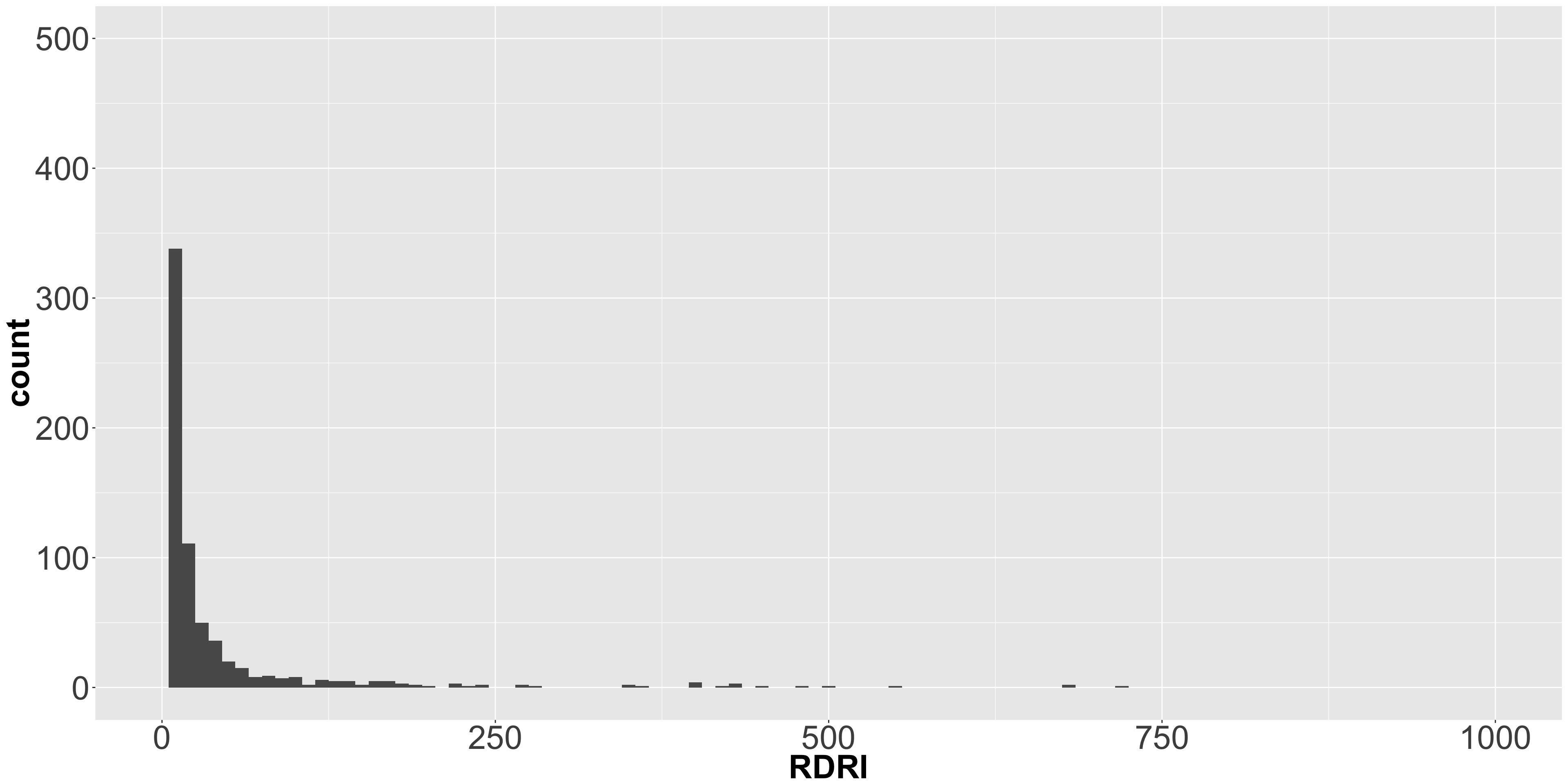
## 7 RDRI 3.11 30.79 0A glance at the RDRI quantiles shows that this variation is due to relatively few packages. The histogram indicates a very long tail.
quantile(c_dat$RDRI)## 0% 25% 50% 75% 100%
## 0 0 0 0 1239## Warning: Removed 4 rows containing non-finite values (stat_bin).## Warning: Removed 1 rows containing missing values (geom_bar).
Sorting the RDRI field finds the top 15 most integrated packages. By this, I mean the packages that are most depended upon or imported by other packages.
top_RDRI <- c_dat %>% arrange(desc(RDRI))
head(top_RDRI[,c(1,2,7,8)],15)
## Package Aut DepImp RDRI
## 1 Rcpp 7 3 1239
## 2 MASS 6 6 1157
## 3 MASS 6 6 1157
## 4 ggplot2 3 11 1149
## 5 dplyr 5 12 716
## 6 Matrix 13 7 680
## 7 Matrix 13 7 680
## 8 plyr 1 2 555
## 9 stringr 2 3 500
## 10 mvtnorm 9 3 483
## 11 magrittr 1 0 454
## 12 survival 2 7 434
## 13 survival 2 7 434
## 14 jsonlite 3 1 426
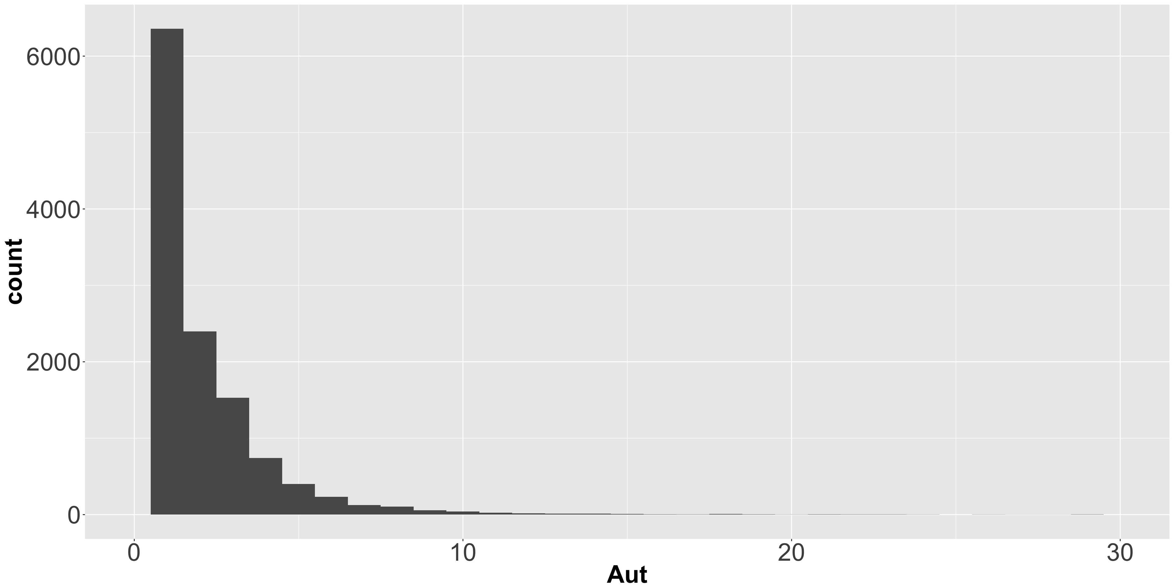
## 15 httr 2 6 420Finally, looking at the quantiles and histogram of the authors field gives some idea of collaboration. Most packages have fewer than three authors, indicating only very modest collaboration.
Author quantiles
quantile(c_dat$Aut)## 0% 25% 50% 75% 100%
## 1 1 1 3 97## Warning: Removed 9 rows containing non-finite values (stat_bin).
I hope the easy availability of package meta data provided by CRAN_package_db() will inspire some serious work on analyzing the characteristics of R packages.
You may leave a comment below or discuss the post in the forum community.rstudio.com.