Writing a domain-specific language (DSL) is a powerful and fairly common method for extending the R language. Both ggplot2 and dplyr, for example, are DSLs. (See Hadley’s chapter in Advanced R for some elaboration.) In this post, I take a first look at NIMBLE (Numerical Inference for Statistical Models using Bayesian and Likelihood Estimation), a DSL for formulating and efficiently solving statistical models in general, and Bayesian hierarchical models in particular. The latter comprise a class of interpretable statistical models useful for both inference and prediction. (See Gelman’s 2006 Technographics paper for what these models can and cannot do.)
Most of what I describe here can be found in the comprehensive and the very readable paper by Valpine et al., or the extensive NIMBLE User Manual.
At the risk of oversimplification, it seems to me that the essence of the NIMBLE is that it is a system for developing models designed around two dichotomies. The first dichotomy is that NIMBLE separates the specification of a model from the implementation of the algorithms that express it. A user can formulate a model in the BUGS language, and then use different NIMBLE functions to solve the model. Or, looking at things the other way round, a user can write a NIMBLE function to implement some algorithm or another efficiently, and then use this function in different models.
The second dichotomy separates model setup from model execution. NIMBLE programming is done by writing nimbleFunctions (see Chapter 11 of the Manual), a subset of the R Language that is augmented with additional data structures and made compilable. nimbleFunctions come in two flavors. Setup functions run once for each model, node any model structure used to define the model. Run functions can be executed by R or compiled into C++ code.
NIMBLE is actually more complicated, or should I say “richer”, than this. There are many advanced programming concepts to wrap your head around. Nevertheless, it is pretty straightforward to start using NIMBLE for models that already have BUGS implementations. The best way to get started for anyone new to Bayesian statistics, or whose hierarchical model building skills may be a bit rusty, is to take the advice of the NIMBLE developers and work through the Pump Model example in Chapter 2 of the manual. In the rest of this post, I present an abbreviated and slightly reworked version of that model.
Before getting started, note that although NIMBLE is an R package listed on CRAN, and it installs like any other R package, you must have a C++ compiler and the standard make utility installed on your system before installing NIMBLE. (See Chapter 4 of the manual for platform-specific installation instructions.)
Pump Failure Model
The Pump Failure model is discussed by George et al. in their 1993 paper: Conjugate Likelihood Distributions. The paper examines Bayesian models that use conjugate priors, but which do not have closed form solutions when prior distributions are associated with the hyperparameters. The BUGS solution of the problem is given here.
The data driving the model are: x[i] the number of failures for pump, i in a time interval, t[i] where i goes from 1 to 10.
library(nimble)
library(igraph)
library(tidyverse)

pumpConsts <- list(N = 10,
t = c(94.3, 15.7, 62.9, 126, 5.24,31.4, 1.05, 1.05, 2.1, 10.5))

pumpData <- list(x = c(5, 1, 5, 14, 3, 19, 1, 1, 4, 22))
Arrival times are a Poisson distribution with parameter lambda, where lambda is itself modeled as a Gamma distribution with hyperparameters alpha and beta.
The model is expressed in the BUGS language wrapped inside the NIMBLE function nimbleCode(), which turns the BUGS code into a object that can be operated on by nimbleModel()
pumpCode <- nimbleCode(
  {
for (i in 1:N){
  theta[i] ~ dgamma(alpha,beta)
  lambda[i] <- theta[i]*t[i]
  x[i] ~ dpois(lambda[i])
  }
alpha ~ dexp(1.0)
beta ~ dgamma(0.1,1.0)
})

pumpInits <- list(alpha = 1, beta = 1,
theta = rep(0.1, pumpConsts$N))
nimbleModel() produces the model object that can be executed by R or compiled.
pump <- nimbleModel(code = pumpCode, name = "pump", constants = pumpConsts,
                    data = pumpData, inits = pumpInits)
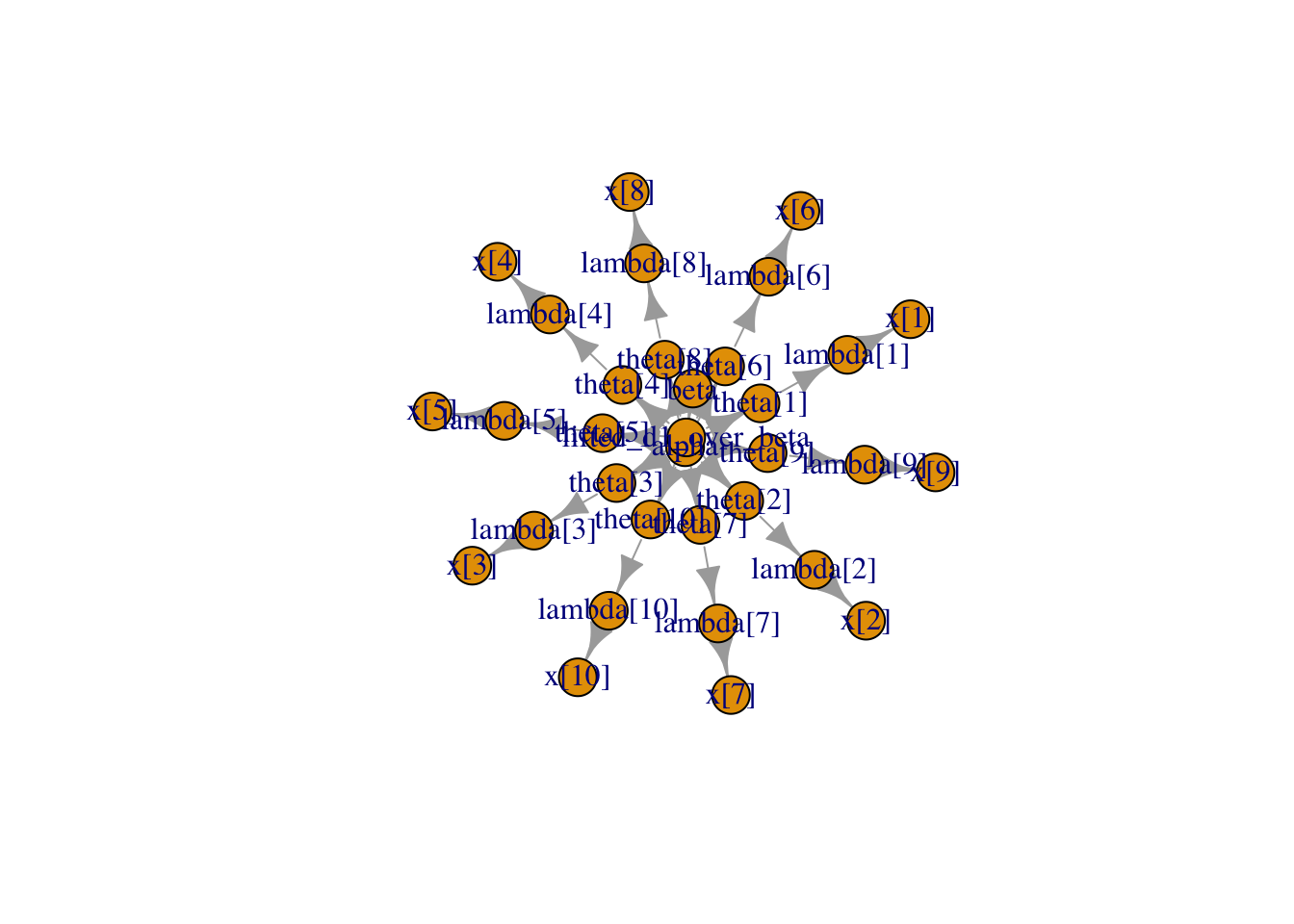
The following command lets us look at the nodes that comprise the model’s directed graph, and plot it.
pump$getNodeNames() [1] "alpha" "beta" "lifted_d1_over_beta"
[4] "theta[1]" "theta[2]" "theta[3]"
[7] "theta[4]" "theta[5]" "theta[6]"
[10] "theta[7]" "theta[8]" "theta[9]"
[13] "theta[10]" "lambda[1]" "lambda[2]"
[16] "lambda[3]" "lambda[4]" "lambda[5]"
[19] "lambda[6]" "lambda[7]" "lambda[8]"
[22] "lambda[9]" "lambda[10]" "x[1]"
[25] "x[2]" "x[3]" "x[4]"
[28] "x[5]" "x[6]" "x[7]"
[31] "x[8]" "x[9]" "x[10]" pump$plotGraph()
We can look at the values stored at each node. The node for x contains the initial values we entered into the model and the nodes for theta and lambda contain the initial calculated values
pump$x [1] 5 1 5 14 3 19 1 1 4 22pump$theta [1] 0.1 0.1 0.1 0.1 0.1 0.1 0.1 0.1 0.1 0.1pump$lambda [1] 9.430 1.570 6.290 12.600 0.524 3.140 0.105 0.105 0.210 1.050We can also look at the log probabilities of the likelihoods.
pump$logProb_x [1] -2.998011 -1.118924 -1.882686 -2.319466 -4.254550 -20.739651
[7] -2.358795 -2.358795 -9.630645 -48.447798Next, we use the model to simulate new values for theta and update the variables.
set.seed(1)
pump$simulate("theta")
pump$theta
[1] 0.15514136 1.88240160 1.80451250 0.83617765 1.22254365 1.15835525
[7] 0.99001994 0.30737332 0.09461909 0.15720154These new values will, of course, lead to new values of lambda and the log probabilities.
pump$lambda [1] 9.430 1.570 6.290 12.600 0.524 3.140 0.105 0.105 0.210 1.050pump$logProb_x [1] -2.998011 -1.118924 -1.882686 -2.319466 -4.254550 -20.739651
[7] -2.358795 -2.358795 -9.630645 -48.447798The model can also be compiled. The C++ code generated is loaded back into R with an object that can be examined like the uncompiled model.
Cpump <- compileNimble(pump)
Cpump$theta
[1] 0.15514136 1.88240160 1.80451250 0.83617765 1.22254365 1.15835525
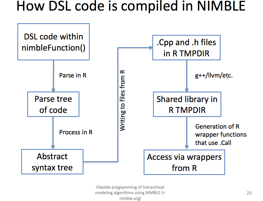
[7] 0.99001994 0.30737332 0.09461909 0.15720154Note that since a wide variety of NIMBLE models can be compiled, NIMBLE should be generally useful for developing production R code. Have a look at the presentation by Christopher Paciorek for a nice overview of NIMBLE’s compilation process.

Next, the default NIMBLE MCMC algorithm is used to generate posterior samples from the distributions for the model parameters alpha, beta, theta and lambda, along with summary statistics and the value of Wantanabi’s WAIC statistic.
mcmc.out <- nimbleMCMC(code = pumpCode, constants = pumpConsts,
                       data = pumpData, inits = pumpInits,
                       monitors=c("alpha","beta","theta","lambda"),
                       nchains = 2, niter = 10000,
                       summary = TRUE, WAIC = TRUE)
|-------------|-------------|-------------|-------------|
|-------------------------------------------------------|
|-------------|-------------|-------------|-------------|
|-------------------------------------------------------|names(mcmc.out)[1] "samples" "summary" "WAIC" The model object contains a summary of the model,
mcmc.out$summary$chain1
Mean Median St.Dev. 95%CI_low 95%CI_upp
alpha 0.69804352 0.65835063 0.27037676 0.287898244 1.3140461
beta 0.92862598 0.82156847 0.54969128 0.183699137 2.2872696
lambda[1] 5.67617535 5.35277649 2.39989346 1.986896247 11.3087435
lambda[2] 1.59476464 1.28802618 1.24109695 0.126649837 4.7635134
lambda[3] 5.58222072 5.28139948 2.36539331 1.961659802 11.1331869
lambda[4] 14.57540796 14.23984600 3.79587390 8.085538041 22.9890092
lambda[5] 3.16402849 2.87859865 1.63590766 0.836991007 7.1477641
lambda[6] 19.21831706 18.86685281 4.33423677 11.703168568 28.6847447
lambda[7] 0.94776605 0.74343559 0.77658191 0.077828283 2.8978174
lambda[8] 0.93472103 0.74313533 0.76301563 0.076199581 2.9598715
lambda[9] 3.31124086 3.03219017 1.61332897 0.955909813 7.2024472
lambda[10] 20.89018329 20.59798130 4.45302924 13.034529765 30.4628012
theta[1] 0.06019274 0.05676327 0.02544956 0.021069950 0.1199230
theta[2] 0.10157737 0.08203988 0.07905076 0.008066869 0.3034085
theta[3] 0.08874755 0.08396502 0.03760562 0.031186960 0.1769982
theta[4] 0.11567784 0.11301465 0.03012598 0.064170937 0.1824525
theta[5] 0.60382223 0.54935089 0.31219612 0.159731108 1.3640771
theta[6] 0.61204831 0.60085518 0.13803302 0.372712375 0.9135269
theta[7] 0.90263434 0.70803389 0.73960182 0.074122175 2.7598261
theta[8] 0.89021051 0.70774794 0.72668155 0.072571029 2.8189252
theta[9] 1.57678136 1.44390008 0.76825189 0.455195149 3.4297368
theta[10] 1.98954127 1.96171250 0.42409802 1.241383787 2.9012192
$chain2
Mean Median St.Dev. 95%CI_low 95%CI_upp
alpha 0.69101961 0.65803654 0.26548378 0.277195564 1.2858148
beta 0.91627273 0.81434426 0.53750825 0.185772263 2.2702428
lambda[1] 5.59893463 5.29143956 2.32153991 1.976164994 10.9564380
lambda[2] 1.57278293 1.27425268 1.23323878 0.129781580 4.7262566
lambda[3] 5.60321125 5.27780200 2.32992322 1.970709123 10.9249502
lambda[4] 14.60674094 14.30971897 3.86145332 8.013012004 23.0526313
lambda[5] 3.13119513 2.84685917 1.67006926 0.782262325 7.2043337
lambda[6] 19.17917926 18.82326155 4.33456380 11.661139736 28.5655803
lambda[7] 0.94397897 0.74446578 0.76576887 0.080055678 2.8813517
lambda[8] 0.94452324 0.74263433 0.77013200 0.074813473 2.9457364
lambda[9] 3.30813061 3.04512049 1.58008544 0.986914665 7.0355869
lambda[10] 20.88570471 20.60384141 4.44130984 13.092562597 30.5574424
theta[1] 0.05937364 0.05611283 0.02461866 0.020956151 0.1161870
theta[2] 0.10017726 0.08116259 0.07855024 0.008266343 0.3010355
theta[3] 0.08908126 0.08390782 0.03704170 0.031330829 0.1736876
theta[4] 0.11592652 0.11356920 0.03064645 0.063595333 0.1829574
theta[5] 0.59755632 0.54329373 0.31871551 0.149286703 1.3748728
theta[6] 0.61080189 0.59946693 0.13804343 0.371373877 0.9097319
theta[7] 0.89902759 0.70901502 0.72930369 0.076243503 2.7441445
theta[8] 0.89954594 0.70727079 0.73345905 0.071250926 2.8054633
theta[9] 1.57530029 1.45005738 0.75242164 0.469959364 3.3502795
theta[10] 1.98911473 1.96227061 0.42298189 1.246910723 2.9102326
$all.chains
Mean Median St.Dev. 95%CI_low 95%CI_upp
alpha 0.69453156 0.65803654 0.26795776 0.28329854 1.2999319
beta 0.92244935 0.81828160 0.54365539 0.18549077 2.2785444
lambda[1] 5.63755499 5.32462511 2.36129857 1.98294712 11.1597721
lambda[2] 1.58377379 1.28149065 1.23719199 0.12734396 4.7382079
lambda[3] 5.59271599 5.28024565 2.34769002 1.96451069 11.0072923
lambda[4] 14.59107445 14.27080924 3.82874035 8.04541916 23.0250158
lambda[5] 3.14761181 2.86460377 1.65311690 0.80506062 7.1718837
lambda[6] 19.19874816 18.84484055 4.33433610 11.68198222 28.6445471
lambda[7] 0.94587251 0.74395440 0.77117739 0.07927988 2.8911629
lambda[8] 0.93962214 0.74299160 0.76657858 0.07571751 2.9470742
lambda[9] 3.30968573 3.03910484 1.59675456 0.97386482 7.1120082
lambda[10] 20.88794400 20.60051118 4.44706278 13.05509616 30.5216406
theta[1] 0.05978319 0.05646474 0.02504028 0.02102807 0.1183433
theta[2] 0.10087731 0.08162361 0.07880204 0.00811108 0.3017967
theta[3] 0.08891440 0.08394667 0.03732417 0.03123228 0.1749967
theta[4] 0.11580218 0.11326039 0.03038683 0.06385253 0.1827382
theta[5] 0.60068928 0.54668011 0.31548032 0.15363752 1.3686801
theta[6] 0.61142510 0.60015416 0.13803618 0.37203765 0.9122467
theta[7] 0.90083096 0.70852800 0.73445465 0.07550465 2.7534885
theta[8] 0.89487822 0.70761105 0.73007484 0.07211191 2.8067373
theta[9] 1.57604083 1.44719278 0.76035931 0.46374515 3.3866706
theta[10] 1.98932800 1.96195345 0.42352979 1.24334249 2.9068229and the value of the WAIC statistic.
mcmc.out$WAI[1] 48.69896Here, we select sample values for the parameters for pump 1 in the first chain, and put them into a data frame for plotting.
df <- data.frame(mcmc.out$samples$chain1)
df_l <- df %>% select(alpha, beta, theta.1., lambda.1.) %>% gather(key="parameter", value="value")
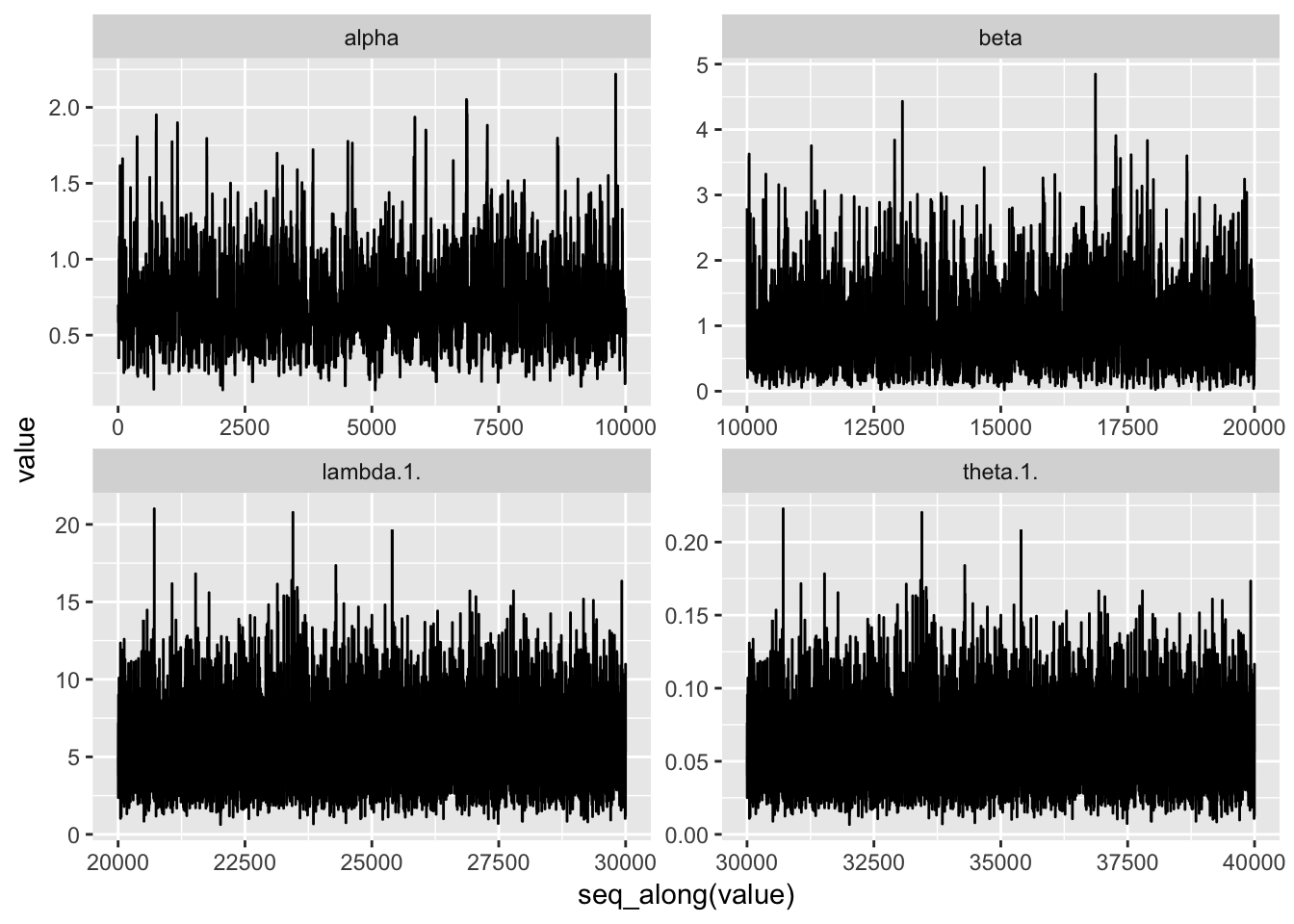
We plot the sample values.
ps <- df_l %>% ggplot(aes(x=seq_along(value), y = value)) + geom_line()
ps + facet_wrap(~parameter, scales = "free")
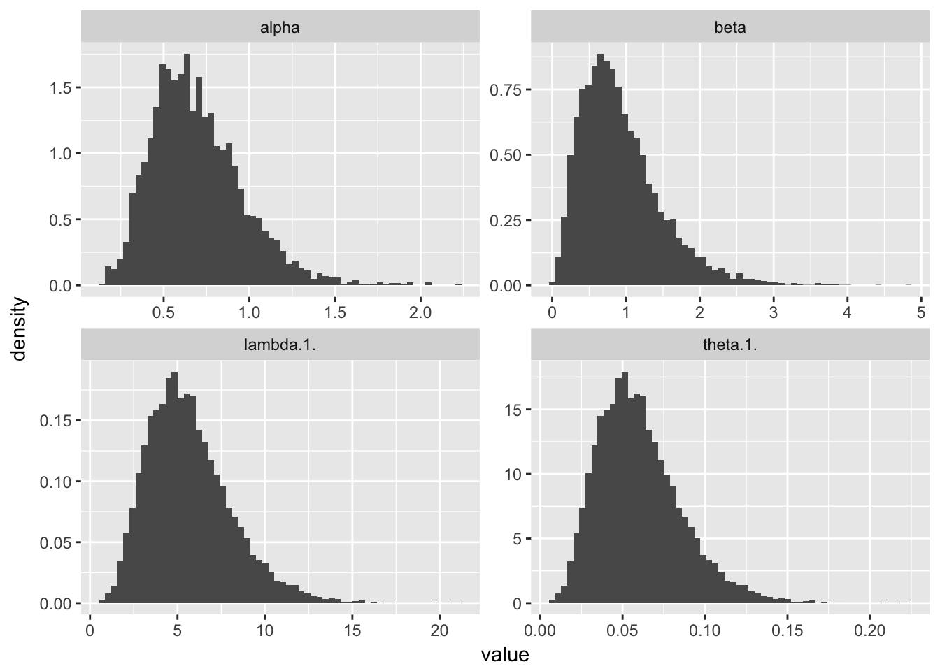
And, we plot histograms.
p <- ggplot(df_l,aes(value)) + geom_histogram(aes( y= ..density..),bins = 60)
p + facet_wrap(~parameter, scales = "free")
Note that it is also possible to perform the MCMC simulation using the compiled model.
mcmc.out_c<- nimbleMCMC(model=Cpump,
                       monitors=c("alpha","beta","theta","lambda"),
                       nchains = 2, niter = 10000,
                       summary = TRUE, WAIC = TRUE)
|-------------|-------------|-------------|-------------|
|-------------------------------------------------------|
|-------------|-------------|-------------|-------------|
|-------------------------------------------------------|mcmc.out_c$summary$chain1
Mean Median St.Dev. 95%CI_low 95%CI_upp
alpha 0.70269965 0.65474666 0.27690796 0.288871669 1.3525877
beta 0.92892181 0.82320341 0.54874194 0.186215812 2.2756643
lambda[1] 5.65646492 5.32568604 2.38108302 1.991839453 11.1329833
lambda[2] 1.58848917 1.28392445 1.25676948 0.133001650 4.7163618
lambda[3] 5.62720720 5.30681963 2.36776285 1.986194548 11.1264464
lambda[4] 14.61256770 14.29447077 3.75584085 8.106535985 22.8405075
lambda[5] 3.16521167 2.88771869 1.65132178 0.785161558 7.0181185
lambda[6] 19.12824948 18.77541823 4.27045427 11.733960316 28.4815908
lambda[7] 0.94353548 0.75312906 0.75111813 0.079570796 2.8410369
lambda[8] 0.93661525 0.74764821 0.75397145 0.078424425 2.8536890
lambda[9] 3.33178422 3.05974419 1.63035789 1.019006182 7.3163945
lambda[10] 20.90388784 20.58355995 4.45456152 12.997984788 30.2815949
theta[1] 0.05998372 0.05647599 0.02525009 0.021122370 0.1180592
theta[2] 0.10117765 0.08177863 0.08004901 0.008471443 0.3004052
theta[3] 0.08946275 0.08436915 0.03764329 0.031577020 0.1768910
theta[4] 0.11597276 0.11344818 0.02980826 0.064337587 0.1812739
theta[5] 0.60404803 0.55109135 0.31513774 0.149839992 1.3393356
theta[6] 0.60917992 0.59794326 0.13600173 0.373693004 0.9070570
theta[7] 0.89860522 0.71726577 0.71535060 0.075781711 2.7057495
theta[8] 0.89201452 0.71204591 0.71806805 0.074689928 2.7177991
theta[9] 1.58656391 1.45702104 0.77636090 0.485241039 3.4839974
theta[10] 1.99084646 1.96033904 0.42424395 1.237903313 2.8839614
$chain2
Mean Median St.Dev. 95%CI_low 95%CI_upp
alpha 0.70184646 0.65773527 0.27237859 0.297108329 1.3420954
beta 0.92323539 0.82124257 0.53880496 0.194879601 2.2590201
lambda[1] 5.59702813 5.25201276 2.35832632 2.029382518 10.9327321
lambda[2] 1.62105397 1.31199418 1.26269004 0.137977536 4.8652461
lambda[3] 5.62874314 5.33611797 2.37576774 1.953756972 11.1296452
lambda[4] 14.53507135 14.22210300 3.84823087 8.042950272 22.9287741
lambda[5] 3.17647361 2.88816158 1.67257096 0.807468793 7.2500264
lambda[6] 19.13576117 18.82011366 4.34294395 11.646448559 28.4716352
lambda[7] 0.94656373 0.74705570 0.76192793 0.084445304 2.9245815
lambda[8] 0.94754678 0.75725106 0.75136514 0.083985118 2.8740656
lambda[9] 3.34514300 3.04989975 1.64818642 0.974288761 7.2961225
lambda[10] 20.97154230 20.61713159 4.45405753 13.260753885 30.5614115
theta[1] 0.05935343 0.05569473 0.02500876 0.021520493 0.1159357
theta[2] 0.10325185 0.08356651 0.08042612 0.008788378 0.3098883
theta[3] 0.08948717 0.08483494 0.03777055 0.031061319 0.1769419
theta[4] 0.11535771 0.11287383 0.03054151 0.063832939 0.1819744
theta[5] 0.60619725 0.55117587 0.31919293 0.154097098 1.3835928
theta[6] 0.60941915 0.59936668 0.13831032 0.370906005 0.9067400
theta[7] 0.90148927 0.71148162 0.72564565 0.080424099 2.7853158
theta[8] 0.90242550 0.72119149 0.71558585 0.079985826 2.7372053
theta[9] 1.59292524 1.45233321 0.78485068 0.463947029 3.4743440
theta[10] 1.99728974 1.96353634 0.42419596 1.262928941 2.9106106
$all.chains
Mean Median St.Dev. 95%CI_low 95%CI_upp
alpha 0.70227305 0.65580594 0.27464608 0.292312894 1.3489184
beta 0.92607860 0.82237274 0.54378998 0.191611561 2.2684771
lambda[1] 5.62674653 5.28611334 2.36985910 2.007150471 11.0415843
lambda[2] 1.60477157 1.29777398 1.25980697 0.135465213 4.8015059
lambda[3] 5.62797517 5.32327502 2.37170950 1.967656654 11.1291530
lambda[4] 14.57381952 14.26247905 3.80241886 8.071801955 22.9002186
lambda[5] 3.17084264 2.88801833 1.66194832 0.798927322 7.1492800
lambda[6] 19.13200533 18.78653361 4.30674559 11.682136284 28.4767857
lambda[7] 0.94504960 0.75003915 0.75652494 0.081865294 2.8859048
lambda[8] 0.94208101 0.75177975 0.75267045 0.080734142 2.8644982
lambda[9] 3.33846361 3.05488924 1.63926902 0.990402148 7.3041714
lambda[10] 20.93771507 20.60497943 4.45432662 13.116940079 30.4162660
theta[1] 0.05966857 0.05605635 0.02513106 0.021284735 0.1170900
theta[2] 0.10221475 0.08266076 0.08024248 0.008628358 0.3058284
theta[3] 0.08947496 0.08463076 0.03770603 0.031282300 0.1769341
theta[4] 0.11566523 0.11319428 0.03017793 0.064061920 0.1817478
theta[5] 0.60512264 0.55114854 0.31716571 0.152467046 1.3643664
theta[6] 0.60929953 0.59829725 0.13715750 0.372042557 0.9069040
theta[7] 0.90004724 0.71432300 0.72049994 0.077966947 2.7484808
theta[8] 0.89722001 0.71598072 0.71682900 0.076889659 2.7280935
theta[9] 1.58974458 1.45470916 0.78060429 0.471620071 3.4781768
theta[10] 1.99406810 1.96237899 0.42422158 1.249232389 2.8967872Monte Carlo Expectation Analysis
To illustrate that NIMBLE is more than just an MCMC engine, the manual example uses NIMBLE’s built-in Monte Carlo Expectation algorithm to maximize the marginal likelihood for alpha and beta. The first step is to set up “box constraints” for the model. Then, the buildMCEM() function is used to construct an MCEM algorithm from a NIMBLE model.
pump2 <- pump$newModel()
box = list( list(c("alpha","beta"), c(0, Inf)))
pumpMCEM <- buildMCEM(model = pump2, latentNodes = "theta[1:10]", boxConstraints = box)
This is how to run the Monte Carlo Expectation model. Note that the authors of the NIMBLE manual point out that these results are within 0.01 of the values obtained by George et al.
pumpMLE <- pumpMCEM$run()|-------------|-------------|-------------|-------------|
|-------------------------------------------------------|
Iteration Number: 1.
Current number of MCMC iterations: 1000.
Parameter Estimates:
alpha beta
0.8130146 1.1125783
Convergence Criterion: 1.001.
|-------------|-------------|-------------|-------------|
|-------------------------------------------------------|
Iteration Number: 2.
Current number of MCMC iterations: 1000.
Parameter Estimates:
alpha beta
0.8148887 1.2323211
Convergence Criterion: 0.02959269.
|-------------|-------------|-------------|-------------|
|-------------------------------------------------------|
Iteration Number: 3.
Current number of MCMC iterations: 1000.
Parameter Estimates:
alpha beta
0.8244363 1.2797908
Convergence Criterion: 0.005418668.
|-------------|-------------|-------------|-------------|
|-------------------------------------------------------|
Monte Carlo error too big: increasing MCMC sample size.
|-------------|-------------|-------------|-------------|
|-------------------------------------------------------|
Iteration Number: 4.
Current number of MCMC iterations: 1250.
Parameter Estimates:
alpha beta
0.8280353 1.2700022
Convergence Criterion: 0.001180319.
|-------------|-------------|-------------|-------------|
|-------------------------------------------------------|
Monte Carlo error too big: increasing MCMC sample size.
|-------------|-------------|-------------|-------------|
|-------------------------------------------------------|
Monte Carlo error too big: increasing MCMC sample size.
|-------------|-------------|-------------|-------------|
|-------------------------------------------------------|
Iteration Number: 5.
Current number of MCMC iterations: 2188.
Parameter Estimates:
alpha beta
0.8268224 1.2794244
Convergence Criterion: 0.000745466.Like the tidyverse, NIBMLE is an ecosystem of DSLs. The BUGS language is extended and used as a DSL for formulation models. nimbleFunctions is a language for writing algorithms that may be used with both BUGS and R. But, unlike the tidyverse, the NIMBLE DSLs are not distributed across multiple packages, but instead wrapped up into the NIMBLE package code.
For more on the design an use of DSLs with R, have a look at the Chapter in Advanced R, or Thomas Mailund’s new book, Domain-Specific Languages in R.
You may leave a comment below or discuss the post in the forum community.rstudio.com.