Today, we will return to the Fama French (FF) model of asset returns and use it as a proxy for fitting and evaluating multiple linear models. In a previous post, we reviewed how to run the FF three-factor model on the returns of a portfolio. That is, we ran one model on one set of returns. Today, we will run multiple models on multiple streams of returns, which will allow us to compare those models and hopefully build a code scaffolding that can be used when we wish to explore other factor models.
Let’s get to it!
We will start by importing daily prices and calculating the returns of our five usual ETFs: SPY, EFA, IJS, EEM and AGG. I covered the logic for this task in a previous post and the code is below.
library(tidyverse)
library(broom)
library(tidyquant)
library(timetk)


symbols <- c("SPY", "EFA", "IJS", "EEM", "AGG")


# The prices object will hold our daily price data.
prices <-
  getSymbols(symbols, src = 'yahoo',
             from = "2012-12-31",
             to = "2017-12-31",
             auto.assign = TRUE,
             warnings = FALSE) %>%
  map(~Ad(get(.))) %>%
  reduce(merge) %>%
  `colnames<-`(symbols)


asset_returns_long <-
  prices %>%
  tk_tbl(preserve_index = TRUE, rename_index = "date") %>%
  gather(asset, returns, -date) %>%
  group_by(asset) %>%
  mutate(returns = (log(returns) - log(lag(returns)))) %>%
  na.omit()


asset_returns_long %>%
  head()
# A tibble: 6 x 3
# Groups: asset [1]
date asset returns
<date> <chr> <dbl>
1 2013-01-02 SPY 0.0253
2 2013-01-03 SPY -0.00226
3 2013-01-04 SPY 0.00438
4 2013-01-07 SPY -0.00274
5 2013-01-08 SPY -0.00288
6 2013-01-09 SPY 0.00254We now have the returns of our five ETFs saved in a tidy tibble called asset_returns_long. Normally we would combine these into one portfolio, but we will leave them as individual assets today so we can explore how to model the returns of multiple assets saved in one data object.
We are going to model those individual assets on the Fama French set of five factors to see if those factors explain our asset returns. Those five factors are the market returns (similar to CAPM), firm size (small versus big), firm value (high versus low book-to-market), firm profitability (high versus low operating profits), and firm investment (high versus low total asset growth). To learn more about the theory behind using these factors, see this article.
Our next step is to import our factor data, and luckily FF make them available on their website. I presented the code showing how to import this data in a previous post on my blog so I won’t go through the steps again, but the code is below.
factors_data_address <-
"http://mba.tuck.dartmouth.edu/pages/faculty/ken.french/ftp/Global_5_Factors_Daily_CSV.zip"

factors_csv_name <- "Global_5_Factors_Daily.csv"

temp <- tempfile()

download.file(
  # location of file to be downloaded
  factors_data_address,
  # where we want R to store that file
  temp,
  quiet = TRUE)


Global_5_Factors <-
  read_csv(unz(temp, factors_csv_name), skip = 6 ) %>%
  rename(date = X1, MKT = `Mkt-RF`) %>%
  mutate(date = ymd(parse_date_time(date, "%Y%m%d")))%>%
  mutate_if(is.numeric, funs(. / 100)) %>%
  select(-RF)

Global_5_Factors %>%
  head()
# A tibble: 6 x 6
date MKT SMB HML RMW CMA
<date> <dbl> <dbl> <dbl> <dbl> <dbl>
1 1990-07-02 0.00700 -0.000600 -0.0031 0.0022 0.0004
2 1990-07-03 0.0018 0.0008 -0.0017 0.0007 0.0004
3 1990-07-04 0.0063 -0.0019 -0.0016 -0.0007 0.000300
4 1990-07-05 -0.0074 0.0031 0.0017 -0.0013 0.000600
5 1990-07-06 0.002 -0.0015 0.0002 0.002 -0.000300
6 1990-07-09 0.00240 0.0018 0.0001 0.0004 -0.00240 Next, we mash asset_returns_long and Global_5_Factors into one data object, using left_join(..., by = "date") because each object has a column called date.
data_joined_tidy <-
  asset_returns_long %>%
  left_join(Global_5_Factors, by = "date") %>%
  na.omit()

data_joined_tidy %>%
  head(5)
# A tibble: 5 x 8
# Groups: asset [1]
date asset returns MKT SMB HML RMW CMA
<date> <chr> <dbl> <dbl> <dbl> <dbl> <dbl> <dbl>
1 2013-01-02 SPY 0.0253 0.0199 -0.0043 0.0028 -0.0028 -0.0023
2 2013-01-03 SPY -0.00226 -0.0021 0.00120 0.000600 0.0008 0.0013
3 2013-01-04 SPY 0.00438 0.0064 0.0011 0.0056 -0.0043 0.0036
4 2013-01-07 SPY -0.00274 -0.0014 0.00580 0 -0.0015 0.0001
5 2013-01-08 SPY -0.00288 -0.0027 0.0018 -0.00120 -0.0002 0.00120We now have a tibble called data_joined_tidy with the asset names in the asset column, asset returns in the returns column, and our five FF factors in the MKT, SMB, HML, RMW and CMA columns. We want to explore whether there is a linear relationship between the returns of our five assets and any/all of the five FF factors. Specifically, we will run several linear regressions, save the results, examine the results, and then quickly visualize the results.
The broom and purrr packages will do a lot of the heavy lifting for us eventually, but let’s start with a simple example: regress the return of one ETF on one of the FF factors. We will use do() for this, which I believe has been declared not a best practice but it’s so irresistibly simple to plunk into the pipes.
data_joined_tidy %>%
  filter(asset == "SPY") %>%
  do(model = lm(returns ~ MKT, data = .))
Source: local data frame [1 x 2]
Groups: <by row>
# A tibble: 1 x 2
asset model
* <chr> <list>
1 SPY <S3: lm>That worked, but our model is stored as a nested S3 object. Let’s use tidy(), glance(), and augment() to view the results.
data_joined_tidy %>%
  filter(asset == "SPY") %>%
  do(model = lm(returns ~ MKT, data = .)) %>%
  tidy(model)
# A tibble: 2 x 6
# Groups: asset [1]
asset term estimate std.error statistic p.value
<chr> <chr> <dbl> <dbl> <dbl> <dbl>
1 SPY (Intercept) 0.000126 0.000100 1.26 0.208
2 SPY MKT 1.02 0.0154 66.0 0 data_joined_tidy %>%
filter(asset == "SPY") %>%
do(model = lm(returns ~ MKT, data = .)) %>%
glance(model)# A tibble: 1 x 12
# Groups: asset [1]
asset r.squared adj.r.squared sigma statistic p.value df logLik
<chr> <dbl> <dbl> <dbl> <dbl> <dbl> <int> <dbl>
1 SPY 0.776 0.776 0.00354 4356. 0 2 5319.
# ... with 4 more variables: AIC <dbl>, BIC <dbl>, deviance <dbl>,
# df.residual <int>data_joined_tidy %>%
filter(asset == "SPY") %>%
do(model = lm(returns ~ MKT, data = .)) %>%
augment(model) %>%
head(5)# A tibble: 5 x 10
# Groups: asset [1]
asset returns MKT .fitted .se.fit .resid .hat .sigma .cooksd
<chr> <dbl> <dbl> <dbl> <dbl> <dbl> <dbl> <dbl> <dbl>
1 SPY 0.0253 0.0199 0.0204 3.17e-4 4.90e-3 7.99e-3 0.00354 7.77e-3
2 SPY -0.00226 -0.0021 -0.00201 1.07e-4 -2.47e-4 9.17e-4 0.00354 2.24e-6
3 SPY 0.00438 0.0064 0.00665 1.36e-4 -2.27e-3 1.47e-3 0.00354 3.02e-4
4 SPY -0.00274 -0.0014 -0.00130 1.04e-4 -1.44e-3 8.59e-4 0.00354 7.07e-5
5 SPY -0.00288 -0.0027 -0.00263 1.11e-4 -2.56e-4 9.82e-4 0.00354 2.56e-6
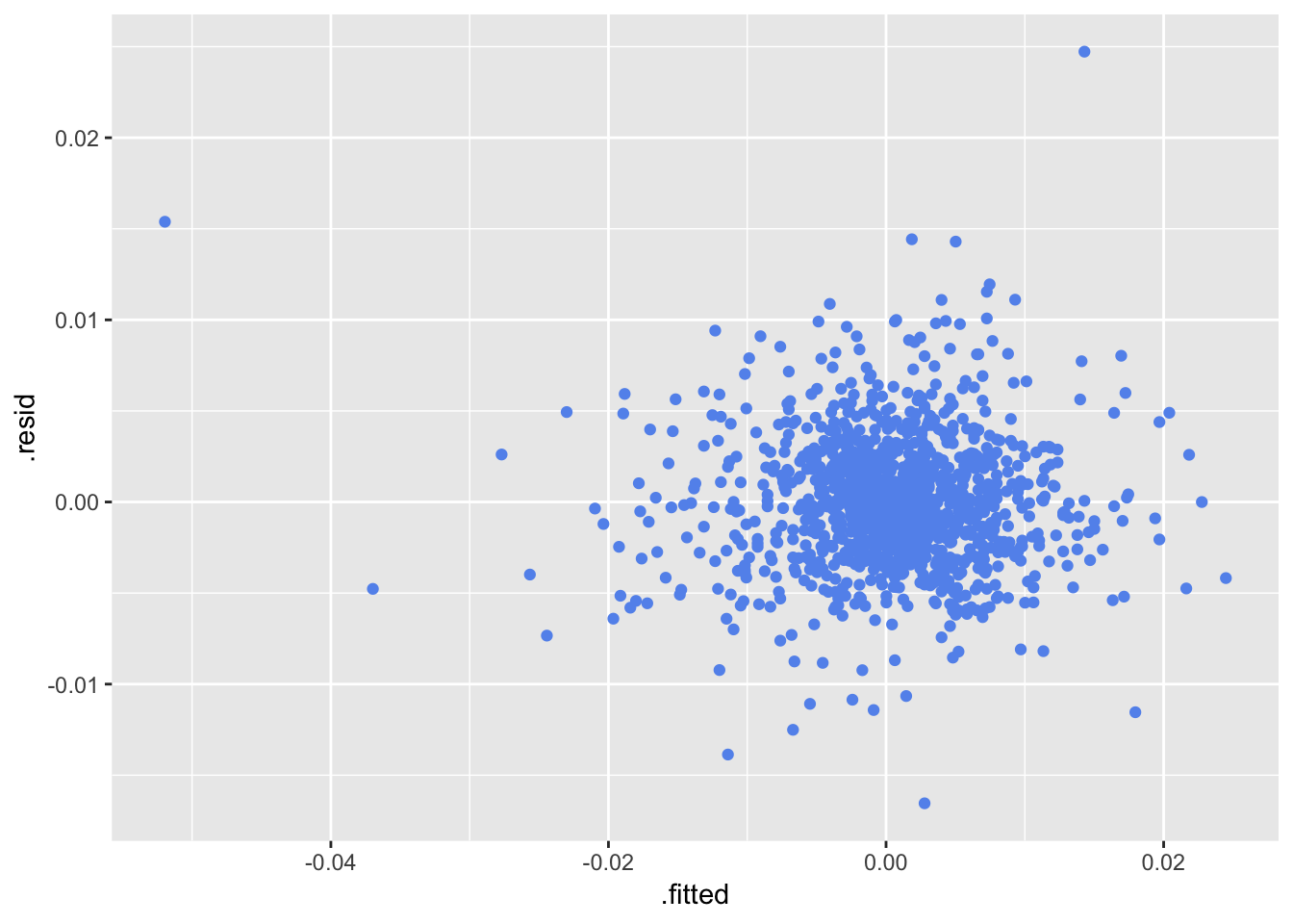
# ... with 1 more variable: .std.resid <dbl>We can quickly pop our augmented results into ggplot() and inspect our residuals versus our fitted values. The important takeaway here is that our augmented results are in a data frame, so we can use all of our ggplot() code flows to create visualizations.
data_joined_tidy %>%
  filter(asset == "SPY") %>%
  do(model = lm(returns ~ MKT, data = .)) %>%
  augment(model) %>%
  ggplot(aes(y = .resid, x = .fitted)) +
  geom_point(color = "cornflowerblue")
Alright, we have run a simple linear regression and seen how tidy(), glance(), and augment() clean up the model results. We could, of course, keep repeating this process for any combination of the FF factors and any of our ETFs, but let’s look at a more efficient approach for fitting multiple models on all of our ETFs.
First, let’s create and save three models as functions. That will allow us to pass them to the map functions from purrr. We will save a one-factor model as a function called model_one, a three-factor model as a function called model_two and a five-factor model as a function called model_three. Note that each function takes a data frame as an argument.
model_one <- function(df) {
  lm(returns ~ MKT, data = df)
}

model_two <- function(df) {
  lm(returns ~ MKT + SMB + HML, data = df)
}

model_three <- function(df) {
  lm(returns ~ MKT + SMB + HML + RMW + CMA, data = df)
}
Now we want to run those three models on each of our five asset returns or, equivalently, we need to pass in a data frame of asset returns to each of those functions. However, we don’t want to save our five ETF returns as five separate tibbles. That would get quite unwieldy with a larger set of ETFs.
Instead, let’s use nest() to make our data more compact!
data_joined_tidy %>%
  group_by(asset) %>%
  nest()
# A tibble: 5 x 2
asset data
<chr> <list>
1 SPY <tibble [1,259 × 7]>
2 EFA <tibble [1,259 × 7]>
3 IJS <tibble [1,259 × 7]>
4 EEM <tibble [1,259 × 7]>
5 AGG <tibble [1,259 × 7]>In my mind, our task has gotten a little conceptually simpler: we want to apply each of our models to each tibble in the data column, and to do that, we need to pass each tibble in that column to our functions.
Let’s use a combination of mutate() and map().
data_joined_tidy %>%
  group_by(asset) %>%
  nest() %>%
  mutate(one_factor_model = map(data, model_one),
         three_factor_model = map(data, model_two),
         five_factor_model = map(data, model_three))
# A tibble: 5 x 5
asset data one_factor_model three_factor_mod… five_factor_mod…
<chr> <list> <list> <list> <list>
1 SPY <tibble [1,25… <S3: lm> <S3: lm> <S3: lm>
2 EFA <tibble [1,25… <S3: lm> <S3: lm> <S3: lm>
3 IJS <tibble [1,25… <S3: lm> <S3: lm> <S3: lm>
4 EEM <tibble [1,25… <S3: lm> <S3: lm> <S3: lm>
5 AGG <tibble [1,25… <S3: lm> <S3: lm> <S3: lm> From a substantive perspective, we’re done! We have run all three models on all five assets and stored the results. Of course, we’d like to be able to look at the results, but the substance is all there.
The same as we did above, we will use tidy(), glimpse(), and augment(), but now in combination with mutate() and map() to clean up the model results stored in each column. Let’s start by running just model_one and then tidying the results.
data_joined_tidy %>%
  group_by(asset) %>%
  nest() %>%
  mutate(one_factor_model = map(data, model_one),
         tidied_one = map(one_factor_model, tidy))
# A tibble: 5 x 4
asset data one_factor_model tidied_one
<chr> <list> <list> <list>
1 SPY <tibble [1,259 × 7]> <S3: lm> <data.frame [2 × 5]>
2 EFA <tibble [1,259 × 7]> <S3: lm> <data.frame [2 × 5]>
3 IJS <tibble [1,259 × 7]> <S3: lm> <data.frame [2 × 5]>
4 EEM <tibble [1,259 × 7]> <S3: lm> <data.frame [2 × 5]>
5 AGG <tibble [1,259 × 7]> <S3: lm> <data.frame [2 × 5]>If we want to see those tidied results, we need to unnest() them.
data_joined_tidy %>%
  group_by(asset) %>%
  nest() %>%
  mutate(one_factor_model = map(data, model_one),
         tidied_one = map(one_factor_model, tidy)) %>%
  unnest(tidied_one)
# A tibble: 10 x 6
asset term estimate std.error statistic p.value
<chr> <chr> <dbl> <dbl> <dbl> <dbl>
1 SPY (Intercept) 0.000126 0.000100 1.26 2.08e- 1
2 SPY MKT 1.02 0.0154 66.0 0.
3 EFA (Intercept) -0.000288 0.0000972 -2.97 3.07e- 3
4 EFA MKT 1.29 0.0150 86.0 0.
5 IJS (Intercept) 0.0000634 0.000171 0.371 7.11e- 1
6 IJS MKT 1.13 0.0264 42.9 3.25e-248
7 EEM (Intercept) -0.000491 0.000203 -2.42 1.57e- 2
8 EEM MKT 1.40 0.0313 44.8 4.94e-263
9 AGG (Intercept) 0.0000888 0.0000572 1.55 1.21e- 1
10 AGG MKT -0.0282 0.00883 -3.19 1.46e- 3Let’s use glance() and augment() as well.
data_joined_tidy %>%
  group_by(asset) %>%
  nest() %>%
  mutate(one_factor_model = map(data, model_one),
         tidied_one = map(one_factor_model, tidy),
         glanced_one = map(one_factor_model, glance),
         augmented_one = map(one_factor_model, augment))
# A tibble: 5 x 6
asset data one_factor_model tidied_one glanced_one augmented_one
<chr> <list> <list> <list> <list> <list>
1 SPY <tibble… <S3: lm> <data.frame… <data.frame… <data.frame […
2 EFA <tibble… <S3: lm> <data.frame… <data.frame… <data.frame […
3 IJS <tibble… <S3: lm> <data.frame… <data.frame… <data.frame […
4 EEM <tibble… <S3: lm> <data.frame… <data.frame… <data.frame […
5 AGG <tibble… <S3: lm> <data.frame… <data.frame… <data.frame […Again, we use unnest() if we wish to look at the glanced or augmented results.
data_joined_tidy %>%
  group_by(asset) %>%
  nest() %>%
  mutate(one_factor_model = map(data, model_one),
         tidied_one = map(one_factor_model, tidy),
         glanced_one = map(one_factor_model, glance),
         augmented_one = map(one_factor_model, augment)) %>%
  # unnest(tidied_one)
   unnest(glanced_one)
# A tibble: 5 x 16
asset data one_factor_model tidied_one augmented_one r.squared
<chr> <list> <list> <list> <list> <dbl>
1 SPY <tibble … <S3: lm> <data.frame … <data.frame [1… 0.776
2 EFA <tibble … <S3: lm> <data.frame … <data.frame [1… 0.855
3 IJS <tibble … <S3: lm> <data.frame … <data.frame [1… 0.594
4 EEM <tibble … <S3: lm> <data.frame … <data.frame [1… 0.615
5 AGG <tibble … <S3: lm> <data.frame … <data.frame [1… 0.00803
# ... with 10 more variables: adj.r.squared <dbl>, sigma <dbl>,
# statistic <dbl>, p.value <dbl>, df <int>, logLik <dbl>, AIC <dbl>,
# BIC <dbl>, deviance <dbl>, df.residual <int> # unnest(augmented_one)data_joined_tidy %>%
group_by(asset) %>%
nest() %>%
mutate(one_factor_model = map(data, model_one),
tidied_one = map(one_factor_model, tidy),
glanced_one = map(one_factor_model, glance),
augmented_one = map(one_factor_model, augment)) %>%
# unnest(tidied_one)
# unnest(glanced_one)
unnest(augmented_one) %>%
head(5)# A tibble: 5 x 10
asset returns MKT .fitted .se.fit .resid .hat .sigma .cooksd
<chr> <dbl> <dbl> <dbl> <dbl> <dbl> <dbl> <dbl> <dbl>
1 SPY 0.0253 0.0199 0.0204 3.17e-4 4.90e-3 7.99e-3 0.00354 7.77e-3
2 SPY -0.00226 -0.0021 -0.00201 1.07e-4 -2.47e-4 9.17e-4 0.00354 2.24e-6
3 SPY 0.00438 0.0064 0.00665 1.36e-4 -2.27e-3 1.47e-3 0.00354 3.02e-4
4 SPY -0.00274 -0.0014 -0.00130 1.04e-4 -1.44e-3 8.59e-4 0.00354 7.07e-5
5 SPY -0.00288 -0.0027 -0.00263 1.11e-4 -2.56e-4 9.82e-4 0.00354 2.56e-6
# ... with 1 more variable: .std.resid <dbl>Let’s change gears a bit and evaluate how well each model explained one of our asset returns, IJS, based on adjusted R-squareds.
First, we use filter(asset == "IJS"), nest the data, then map() each of our models to the nested data. I don’t want the raw data anymore, so will remove it with select(-data).
data_joined_tidy %>%
  group_by(asset) %>%
  filter(asset == "IJS") %>%
  nest() %>%
  mutate(one_factor_model = map(data, model_one),
         three_factor_model = map(data, model_two),
         five_factor_model = map(data, model_three)) %>%
  select(-data)
# A tibble: 1 x 4
asset one_factor_model three_factor_model five_factor_model
<chr> <list> <list> <list>
1 IJS <S3: lm> <S3: lm> <S3: lm> We now have our three model results for the returns of IJS. Let’s use gather() to put those results in tidy format, and then glance() to get at the adjusted R-squared, AIC, and BIC.
models_results <-
  data_joined_tidy %>%
  group_by(asset) %>%
  filter(asset == "IJS") %>%
  nest() %>%
  mutate(one_factor_model = map(data, model_one),
         three_factor_model = map(data, model_two),
         five_factor_model = map(data, model_three)) %>%
  select(-data) %>%
  gather(models, results, -asset) %>%
  mutate(glanced_results = map(results, glance)) %>%
  unnest(glanced_results) %>%
  select(asset, models, adj.r.squared, AIC, BIC)

models_results
# A tibble: 3 x 5
asset models adj.r.squared AIC BIC
<chr> <chr> <dbl> <dbl> <dbl>
1 IJS one_factor_model 0.594 -9282. -9266.
2 IJS three_factor_model 0.599 -9298. -9272.
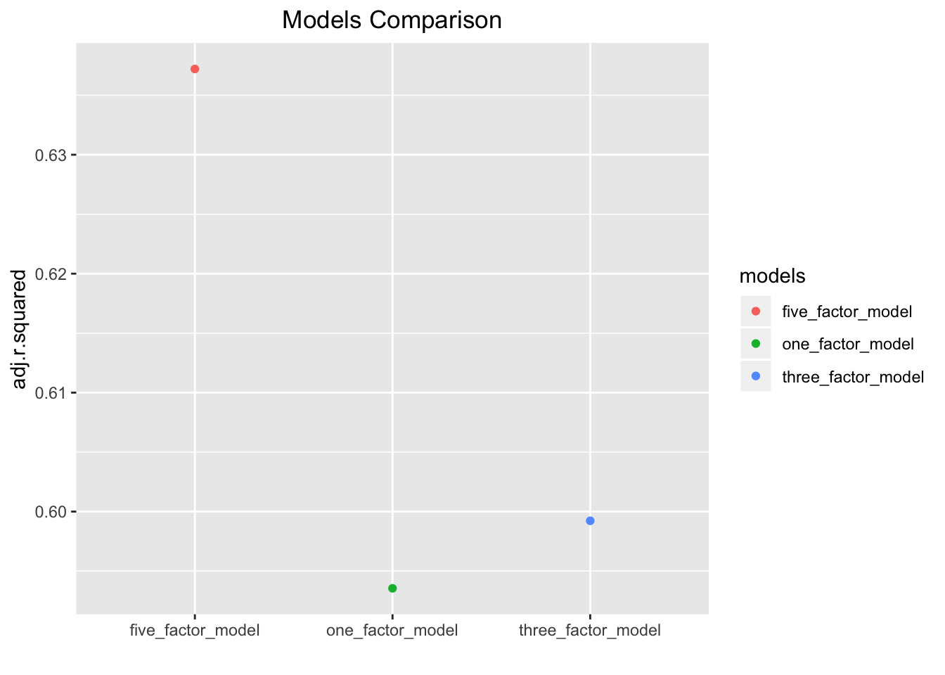
3 IJS five_factor_model 0.637 -9421. -9385.Let’s plot these results and quickly glance at where the adjusted R-squareds lie. We will call ggplot(aes(x = models, y = adj.r.squared, color = models)) and then geom_point().
models_results %>%
  ggplot(aes(x = models, y = adj.r.squared, color = models)) +
  geom_point() +
  labs(x = "",
       title = "Models Comparison") +
  theme(plot.title = element_text(hjust = 0.5))
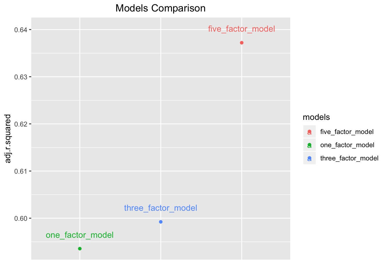
That chart looks alright, but the models are placed on the x-axis in alphabetical order, whereas I’d prefer they go in ascending order based on adjusted R-squared. We can make that happen with ggplot(aes(x = reorder(models, adj.r.squared)...). Let’s also add labels on the chart with geom_text(aes(label = models), nudge_y = .003). Since we’re labeling in the chart, we can remove the x-axis labels with theme(axis.text.x = element_blank()).
models_results %>%
  ggplot(aes(x = reorder(models, adj.r.squared), y = adj.r.squared, color = models)) +
  geom_point(show.legend = NA) +
  geom_text(aes(label = models),
            nudge_y = .003) +
  labs(x = "",
       title = "Models Comparison") +
  theme(plot.title = element_text(hjust = 0.5),
        axis.text.x = element_blank(),
        axis.ticks.x=element_blank())
Pay close attention to the scale on the y-axis. The lowest adjusted R-squared is less than .05 away from the highest. Maybe that amount is meaningful in your world, and maybe it isn’t.
Before we close, let’s get back to modeling and saving results. Here is the full code for running each model on each asset, then tidying, glancing, and augmenting those results. The result is a compact, nested tibble where the columns can be unnested depending on which results we wish to extract.
data_joined_tidy %>%
  group_by(asset) %>%
  nest() %>%
  mutate(one_factor_model = map(data, model_one),
         three_factor_model = map(data, model_two),
         five_factor_model = map(data, model_three)) %>%
  mutate(tidied_one = map(one_factor_model, tidy),
         tidied_three = map(three_factor_model, tidy),
         tidied_five = map(five_factor_model, tidy)) %>%
  mutate(glanced_one = map(one_factor_model, glance),
         glanced_three = map(three_factor_model, glance),
         glanced_five = map(five_factor_model, glance)) %>%
  mutate(augmented_one = map(one_factor_model, augment),
         augmented_three = map(three_factor_model, augment),
         augmented_five = map(five_factor_model, augment)) # %>%
# A tibble: 5 x 14
asset data one_factor_model three_factor_mod… five_factor_mod…
<chr> <list> <list> <list> <list>
1 SPY <tibble [1,25… <S3: lm> <S3: lm> <S3: lm>
2 EFA <tibble [1,25… <S3: lm> <S3: lm> <S3: lm>
3 IJS <tibble [1,25… <S3: lm> <S3: lm> <S3: lm>
4 EEM <tibble [1,25… <S3: lm> <S3: lm> <S3: lm>
5 AGG <tibble [1,25… <S3: lm> <S3: lm> <S3: lm>
# ... with 9 more variables: tidied_one <list>, tidied_three <list>,
# tidied_five <list>, glanced_one <list>, glanced_three <list>,
# glanced_five <list>, augmented_one <list>, augmented_three <list>,
# augmented_five <list> # unnest any broomed column for viewing
# unnest(Insert nested column name here)There are probably more efficient ways to do this, and in the future we’ll explore a package that runs these model comparisons for us, but for now, think about how we could wrap this work to a Shiny application or extend this code flow to accommodate more models and more assets.
Thanks for reading and see you next time!
You may leave a comment below or discuss the post in the forum community.rstudio.com.