Statistics in Glaucoma: Part I

Introduction

Glaucoma is a leading cause of blindness worldwide, with a prevalence of 4% in the population aged 40-80. The disease is characterized by retinal ganglion cell death and corresponding damage to the optic nerve head. Since visual impairment caused by glaucoma is irreversible and efficient treatments exist, early detection of the disease is essential. Determining if the disease is progressing remains one of the most challenging aspects of glaucoma management, since it is difficult to distinguish true progression from variability due to natural degradation or noise. In practice, clinicians monitor progression using a multifactorial approach that relies on various measurements of the disease. In this series of blog posts, we focus on the use of visual fields. Visual field examinations obtain levels of a patient’s actual vision, and the practice is thus referred to as a functional measurement. As such, visual fields are a proxy for a patient’s quality of life, and therefore are typically prioritized in practice.

Visual Field Data

Visual fields are complex spatiotemporal data generated from an intricate anatomical system, which is important to understand for modeling purposes. To illustrate visual field data, we load an example data set from the womblR package on CRAN. The package womblR was developed specifically for analyzing visual field data, and uses a Bayesian hierarchical model that accounts for the complex nature of the data (more details will be provided in Part II). The specific data set comes from the Vein Pulsation Study Trial in Glaucoma and the Lions Eye Institute trial registry, Perth, Western Australia. We begin by loading the package.

library(womblR)

The data set of interest is loaded lazily and can be accessed as follows; we also view the first six rows for illustration.

data(VFSeries)
head(VFSeries)

##   Visit DLS Time Location
## 1     1  25    0        1
## 2     2  23  126        1
## 3     3  23  238        1
## 4     4  23  406        1
## 5     5  24  504        1
## 6     6  21  588        1

The data object VFSeries contains a longitudinal series of visual fields for a glaucoma patient that we will use throughout the three blog posts to exemplify the study of visual fields. This patient has been determined to be progressing, based on the expertise of two clinicians. VFSeries has four variables: Visit, DLS, Time, and Location. The variable Visit represents the visual field test visit number, DLS the observed measure, Time the time of the visual field test (in days from baseline visit), and Location the spatial location on the visual field where the observation occurred. There are 9 visual field exams contained in this data set, and on average 117.25 days between visits.

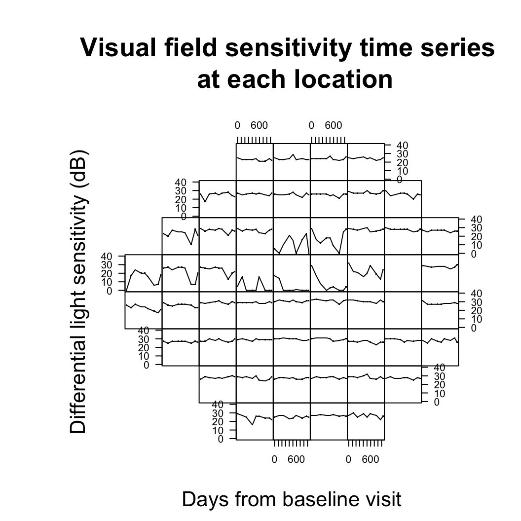
To help visualize the dataframe, we can use the PlotVFTimeSeries function. PlotVFTimeSeries is a function that plots a patient’s observed visual acuity over time at each location on the visual field.

PlotVfTimeSeries(Y = VFSeries$DLS,
                 Location = VFSeries$Location,
                 Time = VFSeries$Time,
                 main = "Visual field sensitivity time series \n at each location",
                 xlab = "Days from baseline visit",
                 ylab = "Differential light sensitivity (dB)",
                 line.reg = FALSE)

The above figure demonstrates the visual field from a Humphrey Field Analyzer-II (HFA-II) testing machine, which generates 54 spatial locations (only 52 informative locations; note the 2 blanks spots corresponding to the blind spot). The visual field map is constructed by assessing a patient’s response to varying levels of light. Patients are instructed to focus on a central fixation point as light is introduced randomly in a preceding manner over a grid on the visual field. As light is observed, the patient presses a button and the current light intensity is recorded. The process is repeated until the entire visual field is tested. The light intensity is measured in differential light sensitivity (DLS), which quantifies the difference in the HFA-II background and observed light intensity. Smaller values indicate worsening vision.

Spatial Anatomy on the Visual Field

The spatial surface of the visual field is observed on a lattice (i.e., uniform areal data); however, it is a complex projection of the underlying optic nerve head and exhibits anatomically induced spatial dependencies. In particular, localized damage to the optic disc can result in clinically deterministic deterioration across the visual field. Incorporating this non-standard spatial dependence structure into our methodology is a priority for properly analyzing these data, although it is commonly ignored. Translating this into math lingo, this means that a naive modeling of the spatial surface of the visual field would be inappropriate (i.e., neighbors defined through adjacent locations). Instead, the definition of a neighbor when considering vision loss on the visual field must depend on the underlying anatomical proximities.

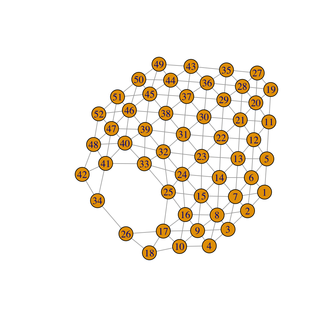
To illustrate this concept, we begin by displaying the visual field neighborhood structure. The adjacency matrix for the HFA-II is available in the womblR package. In this analysis, we use a queen specification, meaning that an adjacency is defined as any location that shares an edge or corner on the lattice. We now load this adjacency matrix and remove the two locations that correspond to the blind spot.

blind_spot <- c(26, 35) # define blind spot
W <- HFAII_Queen[-blind_spot, -blind_spot] # HFA-II visual field adjacency matrix

This adjacency structure can be displayed using the graph.adjacency function in the igraph package.

library(igraph)
adj.graph <- graph.adjacency(W, mode = "undirected") 
plot(adj.graph)

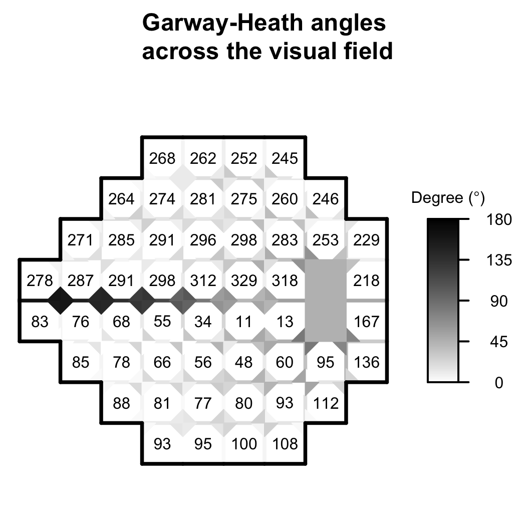
As mentioned above, naively assuming that all of these adjacencies are equal ignores the important underlying anatomy that enforces these dependencies. This anatomical relationship of the visual field test points and the underlying optic nerve head was studied by Garway-Heath et al. (2000), in which they estimated the angle that each test location’s underlying retinal ganglion cells enters the optic disc, measured in degrees. These angles are the missing link that will allow the visual field adjacency structure to be dictated by the underlying anatomy. These angles can be visualized using the function PlotAdjacency from womblR, which displays neighborhood structures across the visual field. Before using this function, we need to load the angles measured in Garway-Heath et al. (2000). These are available from womblR; again, we remove the blind spot before using.

Angles <- GarwayHeath[-blind_spot] # Garway-Heath angles
summary(Angles)

##    Min. 1st Qu.  Median    Mean 3rd Qu.    Max. 
##   11.00   80.75  192.50  177.35  275.75  329.00

We are now ready to visualize the neighborhood structure of the visual field using the PlotAdjacency function.

###Plot the angles on the visual field
PlotAdjacency(W = W, 
              DM = Angles, 
              zlim = c(0, 180), 
              Visit = NA, 
              edgewidth = 3.75,
              cornerwidth = 0.33,
              lwd.border = 3.75,
              main = "Garway-Heath angles\n across the visual field")

The angles measured by Garway-Heath et al. are presented at each location on the visual field. More interestingly, the distances between these angles are presented for each of the neighbor pairs. This figure is equivalent to the adjacency plot displayed above, but allows the adjacencies to vary as a function of the anatomy. In particular, if two visual field locations are anatomically similar, the dependency is strengthened (i.e., more white), and if the locations are close to anatomically independent, the dependency is weaker (i.e., more black). Here the edge adjacencies are represented by lines, while the diagonal adjacencies are represented as two triangles. This view of the visual field details the anatomical importance in modeling visual field data, as neighboring locations can have underlying retinal ganglion cells that enter the optic nerve head with a large degree of separation. In particular, locations on either side of the equator, although adjacent, are anatomically close to independent based on anatomy.

How to Model Visual Field Data?

If you have gotten this far in the post, hopefully you have the sense that the study of visual field data is statistically interesting and clinically important for properly assessing a glaucoma patient’s risk of vision loss. In the next two blog posts, we will explore how visual field data are currently analyzed and new methods that account for the anatomical structure detailed above. To accomplish this, we will break down the algorithm and software used to build the womblR package, and will attempt to illustrate the importance of R packages for open-source clinical research.

Reference

1. Garway-Heath, David F., Darmalingum Poinoosawmy, Frederick W. Fitzke, and Roger A. Hitchings. “Mapping the visual field to the optic disc in normal tension glaucoma eyes” Ophthalmology 107, no. 10 (2000): 1809-1815.