As data scientists, we are often presented with a dataset and are asked to use it to produce insights. We use R to wrangle, visualize, model, and produce tables and plots for sharing or publication. When we focus on the data in hand in this way, we don’t get to consider where the data came from. The sample size and the set of variables and their scales are fixed. Yet the procedures used to gather or generate them are hugely consequential for how we should analyze the data and also the quality of the insights we can ultimately deliver. Sampling procedures have implications for how the resulting data should be analyzed. For studies that seek to measure causal effects, it matters how some units come to be treated and others left untreated.
Because these processes are so important, we wanted to make a tool that would help data scientists and other researchers imagine their data before they collect it so that any changes to process can be made before it’s too late.
When the data is already collected, the tool allows you to imagine your data before you analyze it. When we make data wrangling and modeling decisions based on the results we find under each procedure, or using model fit statistics, we are vulnerable to the unconscious biases labeled the garden of forking paths or p-hacking that may lead us to select the analysis procedure that produces the best answer. We use the actual data because we don’t have a good substitute: data with the same structure and variables that we have collected.
This post introduces the fabricatr package, whose role in the DeclareDesign suite of packages is to simulate data structure and variables. See this RViews post introducing DeclareDesign and the philosophy behind it. fabricatr helps you to think about your data before you start analysis or even collection. What are the units? How are they structured? What measurements will you take? What are their ranges and how are they correlated? fabricatr can help you simulate mock data before you collect the real data, and test out different estimation strategies without worrying about biasing your inferences.
Imagining your data structure
Most simply, fabricatr will create a single-level data structure given a number of units.
library(fabricatr)
fabricate(N = 100, temp_fahrenheit = rnorm(N, mean = 80, sd = 20))
## Warning: `is_lang()` is deprecated as of rlang 0.2.0.
## Please use `is_call()` instead.
## This warning is displayed once per session.## Warning: `lang_name()` is deprecated as of rlang 0.2.0.
## Please use `call_name()` instead.
## This warning is displayed once per session.| ID | temp_fahrenheit |
|---|---|
| 001 | 56.6 |
| 002 | 46.3 |
| 003 | 90.5 |
| 004 | 75.1 |
| 005 | 85.1 |
| 006 | 102.8 |
Social science data is often hierarchical. For example, schools have classrooms that have students. fabricatr shines here with the add_level command. By default, new levels are nested within the levels above them.
library(fabricatr)
fabricate(
  # five schools
  school  = add_level(N = 5,
  n_classrooms = sample(10:15, N, replace = TRUE)),
  # 10 to 15 classrooms per school
  classroom  = add_level(N = n_classrooms),
  # 15 students per classroom
  student = add_level(N = 15)
  )
## Warning: `lang_modify()` is deprecated as of rlang 0.2.0.
## Please use `call_modify()` instead.
## This warning is displayed once per session.| school | n_classrooms | classroom | student |
|---|---|---|---|
| 1 | 12 | 01 | 001 |
| 1 | 12 | 01 | 002 |
| 1 | 12 | 01 | 003 |
| 1 | 12 | 01 | 004 |
| 1 | 12 | 01 | 005 |
| 1 | 12 | 01 | 006 |
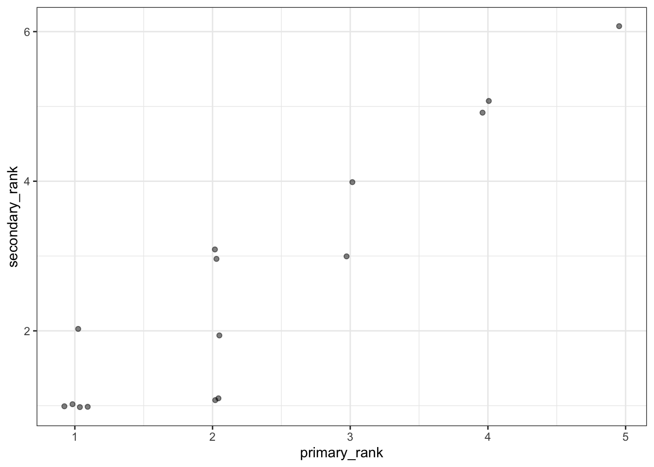
The real world often produces messy, overlapping hierarchies. For example, student data may be collected from middle school and also high school, in which case students are nested in two different schools, but those schools are not nested within each other. Here’s how to make such “cross-classified” data. The rho parameter governs how correlated primary_rank and secondary_rank should be.
dat <-
fabricate(
  primary_schools = add_level(N = 5, primary_rank = 1:N),
  secondary_schools = add_level(N = 6, secondary_rank = 1:N, nest = FALSE),
  students = link_levels(N = 15, by = join(primary_rank, secondary_rank, rho = 0.9))
)
## `link_levels()` calls are faster if the `mvnfast` package is installed.ggplot(dat, aes(primary_rank, secondary_rank)) + geom_point(position = position_jitter(width = 0.1, height = 0.1), alpha = 0.5) + theme_bw()
Similarly, you can create longitudinal data via cross_levels:
fabricate(
 students = add_level(N = 2),
 years = add_level(N = 20, year = 1981:2000, nest = FALSE),
 student_year = cross_levels(by = join(students, years))
)| students | years | year | student_year |
|---|---|---|---|
| 1 | 01 | 1981 | 01 |
| 2 | 01 | 1981 | 02 |
| 1 | 02 | 1982 | 03 |
| 2 | 02 | 1982 | 04 |
| 1 | 03 | 1983 | 05 |
| 2 | 03 | 1983 | 06 |
Imagining your variables
R has lots of great tools for simulating variables. In some cases, though, common kinds of outcome variables are surprisingly tough to simulate. fabricatr collects a small number of functions to create variable types commonly used by social scientists, with simple syntax. We describe two examples here, but see our
variable creation vignette for the rest.
Variables with intra-class correlation
With the data structure tools described above, you can construct data that has
within-unit and between-unit variation, for example, variation within classrooms
and variation across classrooms in test scores. However, many times you want to
set the level of intra-class correlation (ICC) more precisely. We help with
draw_normal_icc and draw_binary_icc.
dat <-
  fabricate(
    N = 1000,
    clusters = sample(LETTERS, N, replace = TRUE),
    Y1 = draw_normal_icc(clusters = clusters, ICC = .2),
    Y2 = draw_binary_icc(clusters = clusters, ICC = .2)
  )
ICC::ICCbare(clusters, Y1, dat)
## [1] 0.09726701ICC::ICCbare(clusters, Y2, dat)## [1] 0.176036Ordered outcomes
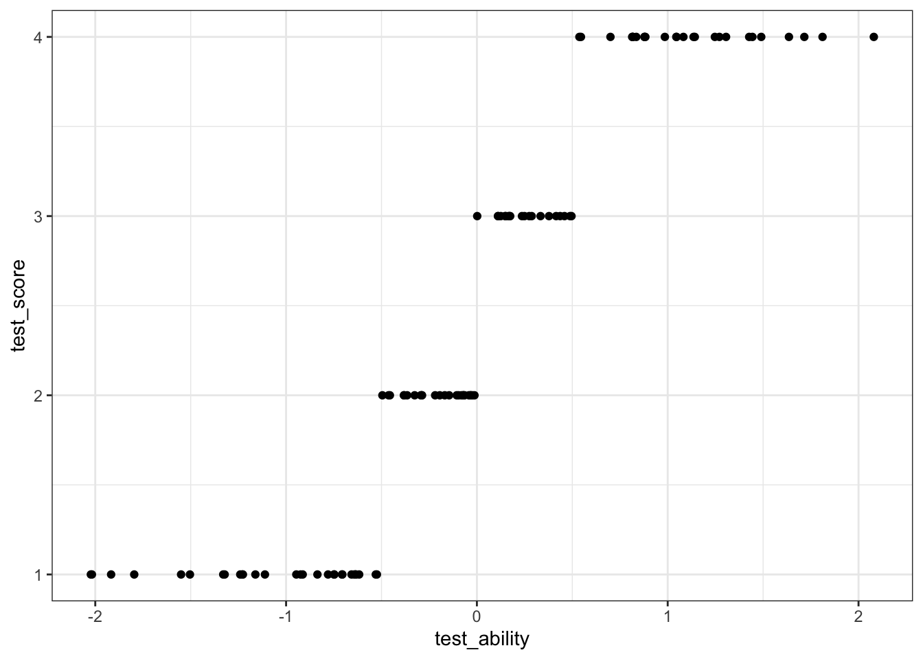
We provide a set of tools for discrete random variables (including ordered outcomes). We take a latent variable (i.e., test_ability) and transform it into an ordered variable (test_score).
dat <-
fabricate(
  N = 100,
  test_ability = rnorm(N),
  test_score = draw_ordered(test_ability, breaks = c(-.5, 0, .5))
)
ggplot(dat, aes(test_ability, test_score)) + geom_point() + theme_bw()
fabricatr is compatible with almost any R variable creation function. We highlight other terrific R packages that help simulate social science-relevant variables in a vignette here.
Where to go next
This post is a high-level teaser for fabricatr’s functionality, but for a deeper introduction, check out the fabricatr getting started vignette. You can also download and print this cheatsheet.
You can install fabricatr from CRAN:
install.packages("fabricatr")
library(fabricatr)
Graeme Blair is an Assistant Professor of Political Science at UCLA.
Jasper Cooper is a Postdoctoral Research Associate at the Kahneman-Treisman Center for Behavioral Science and Public Policy at Princeton University.
Alexander Coppock is an Assistant Professor of Political Science at Yale University.
Macartan Humphreys is a Professor of Political Science at Columbia University and a Director of the research group “Institutions and Political Inequality” at the WZB Berlin Social Science Center.
You may leave a comment below or discuss the post in the forum community.rstudio.com.