Modern Rule-Based Models

Modern Rule-Based Models

Machine learning models come in many shapes and sizes. While deep learning models currently have the lion’s share of coverage, there are many other classes of models that are effective across many different problem domains. This post gives a short summary of several rule-based models that are closely related to tree-based models (but are less widely known).

While this post is focused on explaining on how these models work, it coincides with the release of the rules package, a tidymodels package that provides a user interface to these models. A companion post at the tidyverse blog describes the usage of the package.

To start, let’s discuss the concept of rules more generally.

if (chance_of_rain > 0.75) {
  umbrella <- "yes"
} else {
  umbrella <- "no"
}

for (pkg in c('dplyr', 'modeldata', 'rpart')) {
  if (!requireNamespace(pkg)) {
    install.packages(pkg)
  }
}

library(dplyr)

data(Sacramento, package = "modeldata")

Sacramento <-
  Sacramento %>% 
  mutate(price = log10(price)) %>% 
  select(-zip, -city)

str(Sacramento)

## tibble [932 × 7] (S3: tbl_df/tbl/data.frame)
##  $ beds     : int [1:932] 2 3 2 2 2 3 3 3 2 3 ...
##  $ baths    : num [1:932] 1 1 1 1 1 1 2 1 2 2 ...
##  $ sqft     : int [1:932] 836 1167 796 852 797 1122 1104 1177 941 1146 ...
##  $ type     : Factor w/ 3 levels "Condo","Multi_Family",..: 3 3 3 3 3 1 3 3 1 3 ...
##  $ price    : num [1:932] 4.77 4.83 4.84 4.84 4.91 ...
##  $ latitude : num [1:932] 38.6 38.5 38.6 38.6 38.5 ...
##  $ longitude: num [1:932] -121 -121 -121 -121 -121 ...

library(rpart)

rpart(price ~ ., data = Sacramento) 

## n= 932 
## 
## node), split, n, deviance, yval
##       * denotes terminal node
## 
##  1) root 932 48.5000 5.334  
##    2) sqft< 1594 535 18.7200 5.211  
##      4) sqft< 1170 235  8.0440 5.107  
##        8) sqft< 934.5 71  2.2760 5.002 *
##        9) sqft>=934.5 164  4.6500 5.152 *
##      5) sqft>=1170 300  6.1390 5.292  
##       10) longitude< -121.3 243  4.8850 5.270 *
##       11) longitude>=-121.3 57  0.6081 5.388 *
##    3) sqft>=1594 397 10.6000 5.501  
##      6) sqft< 2317 245  4.7420 5.432  
##       12) longitude< -121.3 205  3.3190 5.407 *
##       13) longitude>=-121.3 40  0.6179 5.562 *
##      7) sqft>=2317 152  2.8450 5.611  
##       14) longitude< -121.2 110  1.6790 5.570 *
##       15) longitude>=-121.2 42  0.4864 5.720 *

if (sqft < 1594 & sqft < 1169.5 & sqft < 934.5) then pred = 5.001820

##  price                                              
##    5.0 when sqft <   935                            
##    5.2 when sqft is  935 to 1170                    
##    5.3 when sqft is 1170 to 1594 & longitude <  -121
##    5.4 when sqft is 1170 to 1594 & longitude >= -121
##    5.4 when sqft is 1594 to 2317 & longitude <  -121
##    5.6 when sqft is 1594 to 2317 & longitude >= -121
##    5.6 when sqft >=         2317 & longitude <  -121
##    5.7 when sqft >=         2317 & longitude >= -121

C5.0 rules

The C4.5 algorithm (Quinlan, 1993b) was an early tree-based model that was released not long after the more well known CART model. One cool aspect of this model is that it could generate a classification tree or a set of rules. These rules are derived from the original tree much in the same way that was shown above for rpart.

Over the years, the author (Ross Quinlan) kept evolving the next generation of the model called C5.0. About 10 years ago, he open-sourced that model and the C50 R package was born. Like its predecessor, C5.0 could be used for trees or for rules. There are a variety of advances to this model (detailed in Kuhn and Johnson (2013)), but the most significant was the inclusion of boosting. In effect, you could create an ensemble of classification rules. Rather than approaching the problem via the more modern stochastic gradient boosting paradigm, it is more similar to the classical AdaBoost methodology.

Since C5.0 is classification only, an example of a single rule set for the iris data is:

Rule 1: (50, lift 2.9)
    Petal.Length <= 1.9
    ->  class setosa  [0.981]

Rule 2: (48/1, lift 2.9)
    Petal.Length > 1.9
    Petal.Length <= 4.9
    Petal.Width <= 1.7
    ->  class versicolor  [0.960]

Rule 3: (46/1, lift 2.9)
    Petal.Width > 1.7
    ->  class virginica  [0.958]

Rule 4: (46/2, lift 2.8)
    Petal.Length > 4.9
    ->  class virginica  [0.938]

Default class: setosa

If used on the iris data, a boosting ensemble with 50 constituent models used a total of 276 rules and each iteration averaged 5.52 rules per rule set.

The primary method of controlling the complexity of each rule set is to adjust the minimum number of data points required to make additional splits within a node. The default for this parameter is two data points. If this value was increased to 20, the mean number of rules was reduced from 5.52 rules to 3.2 rules.

When tuning, the other main tuning parameter is the number of boosting iterations. The C50 R package enables sub-model predictions across boosting iterations; tuning this parameter over many values is not very computation expensive.

Cubist

The aforementioned Ross Quinlan also developed model trees (Quinlan, 1992). These are regression tree-based models that contain linear regression models in the terminal nodes. This model was called M5 and, much like C5.0, there was a rule-based analog. Most tree-based models, especially ensembles of trees, tend to produce models that underfit in the tails (much like regression to the mean). Model trees do not suffer from this issue since their terminal regression models could make predictions across the whole range of the outcome data.

After an initial set of papers in the 1990’s, Quinlan didn’t publish much on the methodology as he evolved it. The modern version of model rules was called Cubist. There were a number of small technical differences between Cubist and M5 rules (enumerated in Kuhn and Johnson (2013)) but the main improvements were:

• An ensemble method for predictions called committees.

• A nearest-neighbor adjustment that occurs after the model predictions.

We’ll summarize these approaches in-turn.

Committee ensembles are similar to boosting. In boosting, a set of models are created sequentially. For the current iteration of boosting, the model is created using case weights that are defined by the results of previous models. In committees, case weights are not changed. Instead the outcome values are modified for each iteration of committees. For example, if a sample is under-predicted previously, its outcome value is changed to be larger so that the model will be pulled upward in an effort to stop under-predicting.

In committees, the first model uses the original outcome value \(y\). On further iterations, a modified value \(y^*\) is used instead. For iteration \(m\), the model uses this adjustment formula:

\[ y^*_{(m)} = y - (\widehat{y}_{(m-1)} - y) \]

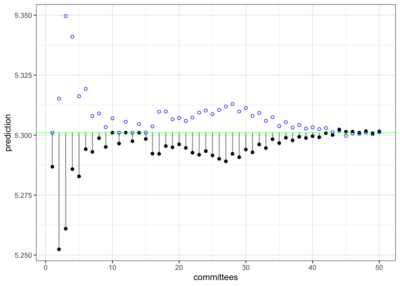
As a demonstration, the plot below shows how the pseudo-outcome changes over iterations. The observed price of the house in question is 5.3. On the first iteration, the model under-predicts (show as the solid black dot). The vertical line represents the residual from this model. On the next iteration, the open blue circle shows the value of \(y^*_{(2)}\). On the second iteration, the prediction for this data point becomes worse but, as iterations proceed, the residuals generally become smaller.

Ensemble predictions are made by averaging over the committee model predictions. This concludes in the model-based prediction made by Cubist.

After the model prediction, there is an option to conduct a post-model nearest-neighbor adjustment (Quinlan, 1993a). When predicting a new data point, the K-nearest neighbors are found in the training set (along with their original predictions). If the training set predictions for the neighbors are denoted as \(t\), the adjustment is:

\[ \widehat{y}_{adj} = \frac{1}{K}\sum_{\ell=1}^K w_\ell \left[t_\ell + \left(\widehat{y} - \widehat{t}_\ell \right)\right] \]

where the weights \(w_\ell\) are based on the inverse distances (so that far points contribute less to the adjustment). The adjustment is large when the difference between the original and new predictions is large. As the difference between the predictions of the new sample and its closest neighbor increases, the adjustment becomes larger.

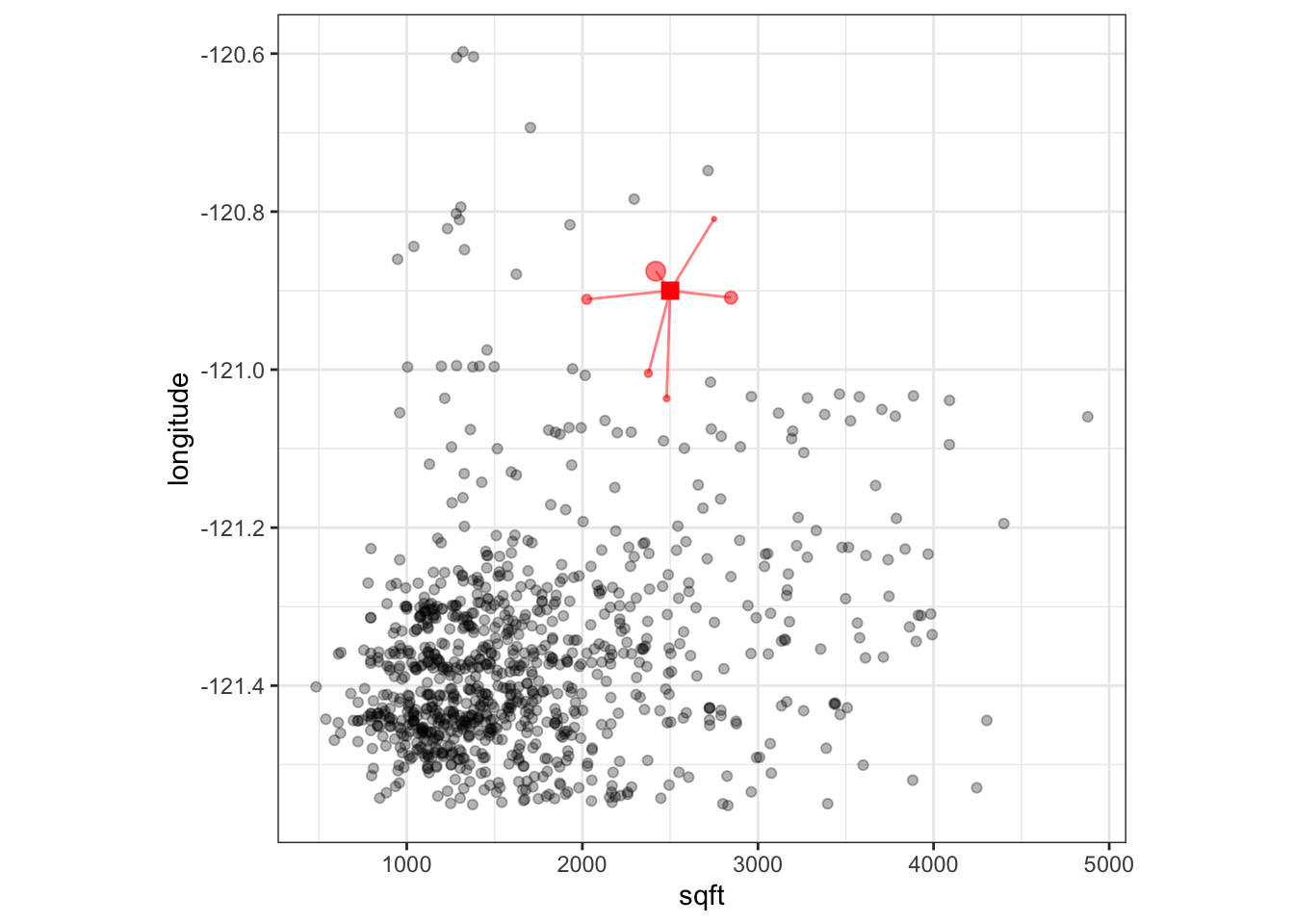
Suppose our model used only square footage and longitude as predictors. The training data are shown below with a new prediction point represented as a large red square. The 6-closest neighbors in the training set are shown as red circles. The size of the circle represents the magnitude of the weight. This shows that the nearby points influence the adjustment more than distant points.

This adjustment generally improves performance of the model. Interestingly, there is often a pattern when tuning where the 1-nearest neighbor model does much worse than using no adjustment but two or more neighbors do a much better job. One idea is that the use of a single neighbor is likely overfitting to the training set (as would occur with a more traditional K-NN model).

Using both of these techniques, Cubist tends to produce very competitive in terms of performance. The two primary parameters are the number of committee members and the number of nearest neighbors to use in the adjustment. The Cubist package can use the same fitted model to make predictions across the number of neighbors, so there is little computational cost when tuning this parameter.

For the Sacramento data, a single model (e.g. one committee) consisted of 6 rules, each with its own linear regression model. For example, the first four rules are:

##   Rule 1: [198 cases, mean 5.187264, range 4.681241 to 5.759668, est err 0.131632]
## 
##     if
##  sqft <= 1712
##  latitude > 38.46639
##  latitude <= 38.61377
##  longitude > -121.5035
##     then
##  outcome = -48.838393 + 0.000376 sqft + 1.39 latitude
## 
##   Rule 2: [254 cases, mean 5.220439, range 4.477121 to 5.923762, est err 0.105572]
## 
##     if
##  sqft <= 1712
##  latitude > 38.61377
##  longitude > -121.5035
##  longitude <= -121.0504
##     then
##  outcome = 93.155414 + 0.000431 sqft + 0.78 longitude + 0.16 latitude
## 
##   Rule 3: [90 cases, mean 5.273133, range 4.851258 to 5.580444, est err 0.078920]
## 
##     if
##  sqft <= 1712
##  latitude <= 38.46639
##     then
##  outcome = 15.750124 + 0.000344 sqft + 0.09 longitude - 0.005 beds
##            + 0.005 baths
## 
##   Rule 4: [35 cases, mean 5.340909, range 5.018076 to 5.616476, est err 0.086056]
## 
##     if
##  sqft <= 1712
##  longitude <= -121.5035
##     then
##  outcome = 4.865655 + 0.000357 sqft

New samples being predicted will fall into one or more rule conditions and the final prediction is the average of all of the corresponding linear model predictions.

If the model is run for 50 committees, a total of 271 rules were used across the committees with the average of 5.42 rules per committee member.

RuleFit

RuleFit models (Friedman and Popescu, 2008) are fairly simple in concept: use a tree ensemble to create a large set of rules, use the rules as binary predictors, then fit a regularized model that only includes the most important rule features.

For example, if a boosted tree were used to generate rules, each path through each tree would generate a conditional statement that can be used to define a model predictor (as was shown above for rpart). If an xgboost model with 100 boosting iterations with a limit of three splits were used on the Sacramento data, an initial set of 609 rules were generated. Some examples:

sqft >= 1594

longitude < -121.2 & latitude >= 38.73 & latitude >= 38.86

longitude >= -121.2 & longitude < -121 & baths < 2.75

longitude < -121.3 & sqft >= 1246 & type == "Multi_Family"

Clearly, the rules show some redundancy; there tends to be a significant amount of similarity in the rules.

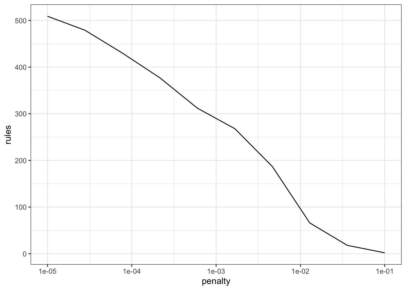
These predictors are added to a regularized regression model (e.g. linear or logistic) that will conduct feature selection to remove unhelpful or redundant rules. Based on how much the model is penalized, the user can choose the number of rules that are contained in the final model. For example, depending on the penalty, the final rule set for the Sacramento data can be as large as hundreds or as small as a handful.

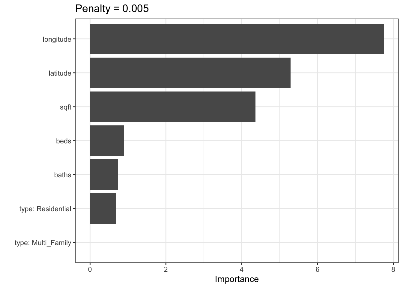
We can generate glmnet variable importance scores and then parameterize the importance in terms of the original predictors (instead of the rules). For example: for a penalty value of \(\lambda\) = 0.005:

RuleFit has many tuning parameters; it inherits them from the boosting model as well as one from glmnet (the amount of lasso regularization). Fortunately, multiple predictions can be made across the lasso penalty using the same model object.

All-in-all, RuleFit is a neat and powerful method for using rules as features. It is interesting to contrast this model and Cubist:

• Cubist creates rules as data subsets then estimates a linear regression models within each.

• RuleFit creates rules as predictors then fits one (generalized) linear model.

Acknowledgments

Ross Quinlan has been supportive of our efforts to publish the inner workings of C5.0 and Cubist. I’d like to thank him for his help and all of the excellent work he has done over the years.

References

Friedman JH; Popescu BE (2008) “Predictive learning via rule ensembles.” _Annals of Applied Statistic_s, pp. 916-954.

Kuhn M; Johnson K (2013) Applied Predictive Modeling, Springer. New York.

Quinlan R (1979). “Discovering rules by induction from large collections of examples.” Expert Systems in the Micro Electronics Age.

Quinlan R (1992). “Learning with continuous classes.” Proceedings of the 5th Australian Joint Conference On Artificial Intelligence, pp. 343-348.

Quinlan R (1993a). “Combining instance-based and model-based learning.” Proceedings of the Tenth International Conference on Machine Learning, pp. 236-243.

Quinlan R (1993b). C4.5: Programs for Machine Learning. Morgan Kaufmann Publishers.