SEM Time Series Modeling

2021-01-22

by Andrea Luciani

Andrea Luciani is a Technical Advisor for the Directorate General for Economics, Statistics and Research at the Bank of Italy, and co-author of the bimets package.

Structural Equation Models (SEM), which are common in many economic modeling efforts, require fitting and simulating whole system of equations where each equation may depend on the results of other equations. Moreover, they often require combining time series and regression equations in ways that are well beyond what the ts() and lm() functions were designed to do. For example, one might want to account for an error auto-correlation of some degree in the regression, or force linear restrictions modeling coefficients.

In this post, we will show how to do structural equation modeling in R by working through the Klein Model of the United States economy, one of the oldest and most elementary models of its kind.

These equations define the model:

$CN_t = \alpha_1 + \alpha_2 * P_t + \alpha_3 * P_{t-1} + \alpha_4 * ( WP_t + WG_t )$

$I_t = \beta_1 + \beta_2 * P_t + \beta_3 * P_{t-1} - \beta_4 * K_{t-1}$

$WP_t = \gamma_1 + \gamma_2 * ( Y_t + T_t - WG_t ) + \gamma_3 * ( Y_{t-1} + T_{t-1} - WG_{t-1} ) + \gamma_4 * Time$

$P_t = Y_t - ( WP_t + WG_t )$

$K_t = K_{t-1} + I_t$

$Y_t = CN_t + I_t + G_t - T_t$

Given:

$CN$ as private consumption expenditure;
$I$ as investment;
$WP$ as wage bill of the private sector (demand for labor);
$P$ as profits;
$K$ as stock of capital goods;
$Y$ as gross national product;
$WG$ as wage bill of the government sector;
$Time$ as an index of the passage of time, e.g. 1931 = zero;
$G$ as government expenditure plus net exports;
$T$ as business taxes.

$\alpha_i, \beta_j, \gamma_k$ are coefficient to be estimated.

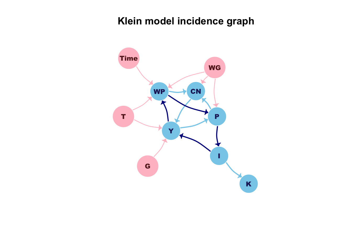
This system has only 6 equations, three of which must be fitted in order to assess the coefficients. It may not seem so difficult to solve this system, but the real complexity emerges if you look at the incidence graph in the following figure, wherein endogenous variables are plotted in blue and exogenous variables are plotted in pink.

Each edge states a simultaneous dependence from a variable to another, e.g. the WP equation depends on the current value of the TIME time series; complexity arises because in this model there are several circular dependencies, one of which is plotted in dark blue.

A circular dependency in the incidence graph of a model implies that the model is a “simultaneous” equations model and that it must be estimated by using ad-hoc procedures; moreover it can be simulated, i.e. performing a forecast, only by using an iterative algorithm.

If we search for “simultaneous equations” inside the Econometrics Task View web page we can find two results: the systemfit and the bimets packages.

The systemfit package is a powerful tool for econometric estimation of simultaneous systems of linear and nonlinear equations, but it only provides fitting procedures, thus it cannot be used in our example in order to work out a forecast.

On the other hand, the bimets package implements, among others, simulation and forecasting procedures; as stated into the vignette it allows users to write down the model in a natural way, to test several strategies and to focus on the econometric analysis, without overly dealing with coding.

Time series projection, linear restrictions and error auto-correlation can be triggered directly in the model definition, so let us try to define a similar but more complex Klein model by using a bimets compliant syntax:

#load library
library(bimets)

#define the Klein model
kleinModelDef <- "
MODEL

COMMENT> Modified Klein Model 1 of the U.S. Economy with PDL, 
COMMENT> autocorrelation on errors, restrictions and conditional equation evaluations

COMMENT> Consumption with autocorrelation on errors
BEHAVIORAL> cn
TSRANGE 1923 1 1940 1
EQ> cn =  a1 + a2*p + a3*TSLAG(p,1) + a4*(wp+wg) 
COEFF> a1 a2 a3 a4
ERROR> AUTO(2)

COMMENT> Investment with restrictions
BEHAVIORAL> i
TSRANGE 1923 1 1940 1
EQ> i = b1 + b2*p + b3*TSLAG(p,1) + b4*TSLAG(k,1)
COEFF> b1 b2 b3 b4
RESTRICT> b2 + b3 = 1

COMMENT> Demand for Labor with PDL
BEHAVIORAL> wp 
TSRANGE 1923 1 1940 1
EQ> wp = c1 + c2*(y+t-wg) + c3*TSLAG(y+t-wg,1) + c4*time
COEFF> c1 c2 c3 c4
PDL> c3 1 2

COMMENT> Gross National Product
IDENTITY> y
EQ> y = cn + i + g - t

COMMENT> Profits
IDENTITY> p
EQ> p = y - (wp+wg)

COMMENT> Capital Stock with IF switches
IDENTITY> k
EQ> k = TSLAG(k,1) + i
IF> i > 0
IDENTITY> k
EQ> k = TSLAG(k,1) 
IF> i <= 0

END
"

#load the model
kleinModel <- LOAD_MODEL(modelText = kleinModelDef)

## Analyzing behaviorals...
## Analyzing identities...
## Optimizing...
## Loaded model "kleinModelDef":
##     3 behaviorals
##     3 identities
##    12 coefficients
## ...LOAD MODEL OK

The code is quite intuitive and uses explicit keywords in order to define equations, coefficients, parameters, etc. Users can easily:

change the TSRANGE in order to fit the model in a custom time range per equation;
modify an equation EQ without changing any user procedure or code;
add or remove one or more linear restriction on the coefficients by using the keyword RESTRICT, e.g.
RESTRICT> -1.23*b2 + 8.9*b3 = 0.34
RESRTICT> b4 – 1.2*b1 = 5
add or remove an error auto-correlation structure with an arbitrary order by using the keyword:
ERROR>

Equations can contain advanced expressions, e.g.:

EQ> TSDELTA(i) = b1 + b2*EXP(p/1000) + b3*TSDELTALOG(TSLAG(p,1)) + b4*MOVAVG(TSLAG(k,1),5)

Model estimation

Now, we define time series to be used in our example, and then we perform an estimation of the whole kleinModel by using the command ESTIMATE():

#define data
kleinModelData <- list(  
  cn  =TIMESERIES(39.8,41.9,45,49.2,50.6,52.6,55.1,56.2,57.3,57.8,
                  55,50.9,45.6,46.5,48.7,51.3,57.7,58.7,57.5,61.6,65,69.7,  
                  START=c(1920,1),FREQ=1),
  g   =TIMESERIES(4.6,6.6,6.1,5.7,6.6,6.5,6.6,7.6,7.9,8.1,9.4,10.7,
                  10.2,9.3,10,10.5,10.3,11,13,14.4,15.4,22.3,   
                  START=c(1920,1),FREQ=1),
  i   =TIMESERIES(2.7,-.2,1.9,5.2,3,5.1,5.6,4.2,3,5.1,1,-3.4,-6.2,
                  -5.1,-3,-1.3,2.1,2,-1.9,1.3,3.3,4.9,  
                  START=c(1920,1),FREQ=1),
  k   =TIMESERIES(182.8,182.6,184.5,189.7,192.7,197.8,203.4,207.6,
                  210.6,215.7,216.7,213.3,207.1,202,199,197.7,199.8,
                  201.8,199.9,201.2,204.5,209.4,    
                  START=c(1920,1),FREQ=1),
  p   =TIMESERIES(12.7,12.4,16.9,18.4,19.4,20.1,19.6,19.8,21.1,21.7,
                  15.6,11.4,7,11.2,12.3,14,17.6,17.3,15.3,19,21.1,23.5, 
                  START=c(1920,1),FREQ=1),
  wp  =TIMESERIES(28.8,25.5,29.3,34.1,33.9,35.4,37.4,37.9,39.2,41.3,
                  37.9,34.5,29,28.5,30.6,33.2,36.8,41,38.2,41.6,45,53.3,    
                  START=c(1920,1),FREQ=1),
  y   =TIMESERIES(43.7,40.6,49.1,55.4,56.4,58.7,60.3,61.3,64,67,57.7,
                  50.7,41.3,45.3,48.9,53.3,61.8,65,61.2,68.4,74.1,85.3, 
                  START=c(1920,1),FREQ=1),
  t   =TIMESERIES(3.4,7.7,3.9,4.7,3.8,5.5,7,6.7,4.2,4,7.7,7.5,8.3,5.4,
                  6.8,7.2,8.3,6.7,7.4,8.9,9.6,11.6, 
                  START=c(1920,1),FREQ=1),
  time=TIMESERIES(NA,-10,-9,-8,-7,-6,-5,-4,-3,-2,-1,0,
                  1,2,3,4,5,6,7,8,9,10, 
                  START=c(1920,1),FREQ=1),
  wg  =TIMESERIES(2.2,2.7,2.9,2.9,3.1,3.2,3.3,3.6,3.7,4,4.2,4.8,
                  5.3,5.6,6,6.1,7.4,6.7,7.7,7.8,8,8.5,  
                  START=c(1920,1),FREQ=1)
);

#load time series into the model object
kleinModel <- LOAD_MODEL_DATA(kleinModel,kleinModelData)

## Load model data "kleinModelData" into model "kleinModelDef"...
## ...LOAD MODEL DATA OK

#estimate the model
kleinModel <- ESTIMATE(kleinModel, quietly=TRUE)

In order to reduce this blog post length we only show the output for a single estimation; anyhow, for each estimated equation the output is similar to the following:

kleinModel <- ESTIMATE(kleinModel, eqList='cn')

## 
## Estimate the Model kleinModelDef:
## the number of behavioral equations to be estimated is 1.
## The total number of coefficients is 4.
## 
## _________________________________________
## 
## BEHAVIORAL EQUATION: cn
## Estimation Technique: OLS
## Autoregression of Order  2  (Cochrane-Orcutt procedure)
## 
## Convergence was reached in  6  /  20  iterations.
## 
## 
## cn                  =   14.83    
##                         T-stat. 7.608    ***
## 
##                     +   0.2589   p
##                         T-stat. 2.96     *
## 
##                     +   0.01424  TSLAG(p,1)
##                         T-stat. 0.1735   
## 
##                     +   0.839    (wp+wg)
##                         T-stat. 14.68    ***
## 
## ERROR STRUCTURE:  AUTO(2) 
## 
## AUTOREGRESSIVE PARAMETERS:
## Rho          Std. Error   T-stat.      
##  0.2542       0.2589       0.9817       
## -0.05251      0.2594      -0.2024       
## 
## 
## STATs:
## R-Squared                      : 0.9827   
## Adjusted R-Squared             : 0.9755   
## Durbin-Watson Statistic        : 2.256    
## Sum of squares of residuals    : 8.072    
## Standard Error of Regression   : 0.8201   
## Log of the Likelihood Function : -18.32   
## F-statistic                    : 136.2    
## F-probability                  : 3.874e-10
## Akaike's IC                    : 50.65    
## Schwarz's IC                   : 56.88    
## Mean of Dependent Variable     : 54.29    
## Number of Observations         : 18
## Number of Degrees of Freedom   : 12
## Current Sample (year-period)   : 1923-1 / 1940-1
## 
## 
## Signif. codes:   *** 0.001  ** 0.01  * 0.05  
## 
## 
## ...ESTIMATE OK

The ESTIMATE() function can fit also non-simultaneous system and a single equation. Several predefined time series transformations are available in bimets:

– Time series extension TSEXTEND()
– Time series merging TSMERGE()
– Time series projection TSPROJECT()
– Lag TSLAG()
– Lag differences: standard, percentage and logarithmic, i.e. TSDELTA(), TSDELTAP(), TSDELTALOG()
– Cumulative product CUMPROD()
– Cumulative sum CUMSUM()
– Moving average MOVAVG()
– Moving sum MOVSUM()
– Parametric (Dis)Aggregation YEARLY(), QUARTERLY(), MONTHLY(), DAILY()
– Time series data presentation TABIT()

Forecasting

The predict() function of the lm() or dyn$lm linear model framework produces predicted values, obtained by evaluating the regression function with new data: it is a popular function among the R users.

Unfortunately, it does not help in our example: as we said before, in order to forecast a simultaneous model that presents circular dependencies in the incidence graph, we cannot merely assess the right-hand side of the equations, as the predict.lm function does; in our case we need an iterative algorithm.

The predict.lm equivalent function that allows to forecast our simultaneous model is the SIMULATE() function. On the other hand the SIMULATE() function can also solve non-simultaneous models and gives the same results as the predict.lm function.

In addition, as in the Capital Stock k equation in our example, the SIMULATE() function can conditionally evaluate an identity during a simulation, depending on the value of a logical expression (e.g. for each simulation period the k equation changes depending on the i current value). Thus, it is possible to have a model alternating between two or more equation specifications for each simulation period, depending upon results from other equations.

Structural stability, multiplier analysis and endogenous targeting are additional capabilities coded in bimets but not described in this post.

In order to forecast the model up to 1944, we need to extend exogenous time series by using the TSEXTEND() function. In this example, we perform simple extensions:

#we need to extend exogenous variables up to 1944
kleinModel$modelData <- within(kleinModel$modelData,{
    wg    = TSEXTEND(wg,  UPTO=c(1944,1),EXTMODE='CONSTANT')
    t     = TSEXTEND(t,   UPTO=c(1944,1),EXTMODE='LINEAR')
    g     = TSEXTEND(g,   UPTO=c(1944,1),EXTMODE='CONSTANT')
    k     = TSEXTEND(k,   UPTO=c(1944,1),EXTMODE='LINEAR')
    time  = TSEXTEND(time,UPTO=c(1944,1),EXTMODE='LINEAR')
  })

A call to the SIMULATE() function will solve our simultaneous system of equations:

#forecast model
kleinModel <- SIMULATE(kleinModel
                      ,simType='FORECAST'
                      ,TSRANGE=c(1941,1,1944,1)
                      ,simConvergence=0.00001
                      ,simIterLimit=100
                      ,quietly=TRUE
  )

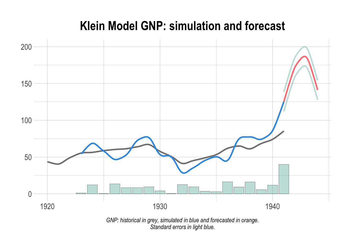
The historical GNP (original referred as “Net national income, measured in billions of 1934 dollars” , pg. 141 in “Economic Fluctuations in the United States 1921-1941” by L. R. Klein, Wiley and Sons Inc., New York, 1950) is shown in figure, along with the simulation and the forecast.

#get forecasted GNP
TABIT(kleinModel$simulation$y)

## 
##       DATE, PER, kleinModel$simulation$y
## 
##       1941, 1  ,  125.3      
##       1942, 1  ,  172.5      
##       1943, 1  ,  185.6      
##       1944, 1  ,  141.1

Disclaimer: The views and opinions expressed in this page are those of the author and do not necessarily reflect the official policy or position of the Bank of Italy. Examples of analysis performed within these pages are only examples. They should not be utilized in real-world analytic products as they are based only on very limited and dated open source information. Assumptions made within the analysis are not reflective of the position of the Bank of Italy.