What does it take to do a t-test?

The two sample t-test

Typically, we have independent samples for some numeric variable of interest (say the concentration of a drug in the blood stream) from two different groups, and we would like to know whether it is likely that two groups differ with respect to this variable. The formal test of the null hypothesis, \(H_0\), that the means of the underlying populations from which the samples are drawn are equal, proceeds making some assumptions:

1. \(H_0\) is true
2. The samples are independent
3. The data are normally distributed
4. The variances of the two samples are equal (This is the simplest test.)

Next, a test statistic that includes the difference between the two sample means is calculated, and a decision is made to establish a “rejection region” for the test statistic. This region depends on the particular circumstances of the test, and is selected to balance the error of rejecting \(H_0\) when it is true against the error of not rejecting \(H_0\) when it is false. If we compute the test statistic and its value does not fall in the rejection region, then we do not reject \(H_0\) and we conclude that we have found nothing. On the other hand, if the test statistic does fall in the rejection region, then we reject the \(H_0\) and conclude that our data along with the the bundle of assumptions we made in setting up the test, and the “steel trap” logic of the t-test itself provide some evidence that the population means are different. (Page 6 of the MIT Open Courseware notes Null Hypothesis Significance Testing II contains an elegantly concise mathematical description of the t-test.)

All of the above assumptions must hold, or be pretty close to holding for the test to give an accurate result. However in my opinion, from the point of view of statistical practice, assumption 2. is fundamental. There are other tests and workarounds for the situations where 4. doesn’t hold. Assumption 3. is very important, but it is relatively easy to check, and the t-test is robust enough to deal with some deviation from normality. Of course, assumption 1. is important. The whole test depends on it, but this assumption is baked into the software that will run the test.

Independence

Independence, on the other hand can be a show stopper. Checking for independence is the difference between doing statistics and carrying out a mathematical or maybe just a mechanical exercise. It often involves considerable creative thinking and tedious legwork.

So, what do we mean by independent samples or independent data, and how do we go about verifying it? Independence is a mathematical idea, an abstraction from probability theory. Two events A and B are said to be independent events if the probability of both A and B happening equals the product of the probabilities of A and B happening. That is: P(AB) = P(A)P(B).

A more intuitive way to think about it is in terms of conditionally probability. In general, the probability of A happening given that B happens is defined to be:

P(A|B) = P(\(A\bigcap B\)) / P(B)

If A and B are independent then P(A|B) = P(A). That is: B has no influence on whether A happens.

“Independent data” or “independent samples” are both shorthand for data sampled or otherwise resulting from independent probability distributions. Relating the mathematical concept to a real world situation requires a clear idea of the population of interest, considerable domain expertise, and a mental slight of hand that is nicely exposed in the short article What are independent samples?, by the Minitab® folks. They write:

Independent samples are samples that are selected randomly so that its observations do not depend on the values other observations.

Notice what is happening here: what started out as a property of probability distributions has now become a prescription for obtaining data in a way that makes it plausible that we can assume independence for the probability distributions that we imagine govern our data. This is a real magic trick. No procedure for selecting data is ever going to guarantee the mathematical properties of our models. Nevertheless, the statement does show the way to proceed. By systematically tracking down all possibilities for interaction within the sampling process and eliminating the possibilities for one sample to influence another it may be possible to reach confidence that it is plausible to assume that the samples are independent. Because the math says that independent data are not correlated much of the exploratory data analysis involves looking for correlations that would signal dependent data. The Minitab® authors make this clear in the example they offer to illustrate their definition.

For example, suppose quality inspectors want to compare two laboratories to determine whether their blood tests give similar results. They send blood samples drawn from the same 10 children to both labs for analysis. Because both labs tested blood specimens from the same 10 children, the test results are not independent. To compare the average blood test results from the two labs, the inspectors would need to do a paired t-test, which is based on the assumption that samples are dependent.

To obtain independent samples, the inspectors would need to randomly select and test 10 children using Lab A and then randomly select and test a different group of 10 different children using Lab B. Then they could compare the average blood test results from the two labs using a 2-sample t-test, which is based on the assumption that samples are independent.

Nicely said, and to further make their point, I am sure that the authors would agree that if it somehow turned out that the children from lab B happened to be the identical twins of the children in Lab A, they still would not have independent samples.

What happens when samples are not independent

The following example illustrates the consequences of performing a t-test when the independence assumption does not hold. We adapt a method of simulating a bivariate normal distribution with a specified covariance matrix that produces two dependent samples with a specified correlation matrix.

library(tidyverse)
library(ggfortify)
set.seed(9999)

First, we simulate a two uncorrelated samples with 20 observations each and run a two-sided t-test with equal variances. As you would expect, test output shows that there are 38 degrees of freedom and the p-value is large.

rbvn_t<-function (n=20, mu1=1, s1=4, mu2=1, s2=4, rho=0)
{
  X <- rnorm(n, mu1, s1)
  Y <- rnorm(n, mu2 + (s2/s1) * rho *
                (X - mu1), sqrt((1 - rho^2)*s2^2))
  t.test(X,Y, mu=0, alternative = "two.sided", var.equal = TRUE)
}
rbvn_t()

## 
##  Two Sample t-test
## 
## data:  X and Y
## t = 2.1, df = 38, p-value = 0.04
## alternative hypothesis: true difference in means is not equal to 0
## 95 percent confidence interval:
##  0.06266 5.06516
## sample estimates:
## mean of x mean of y 
##    2.9333    0.3694

Now we simulate 10,000 two-sided t-tests with independent samples having 20 observations in each sample.

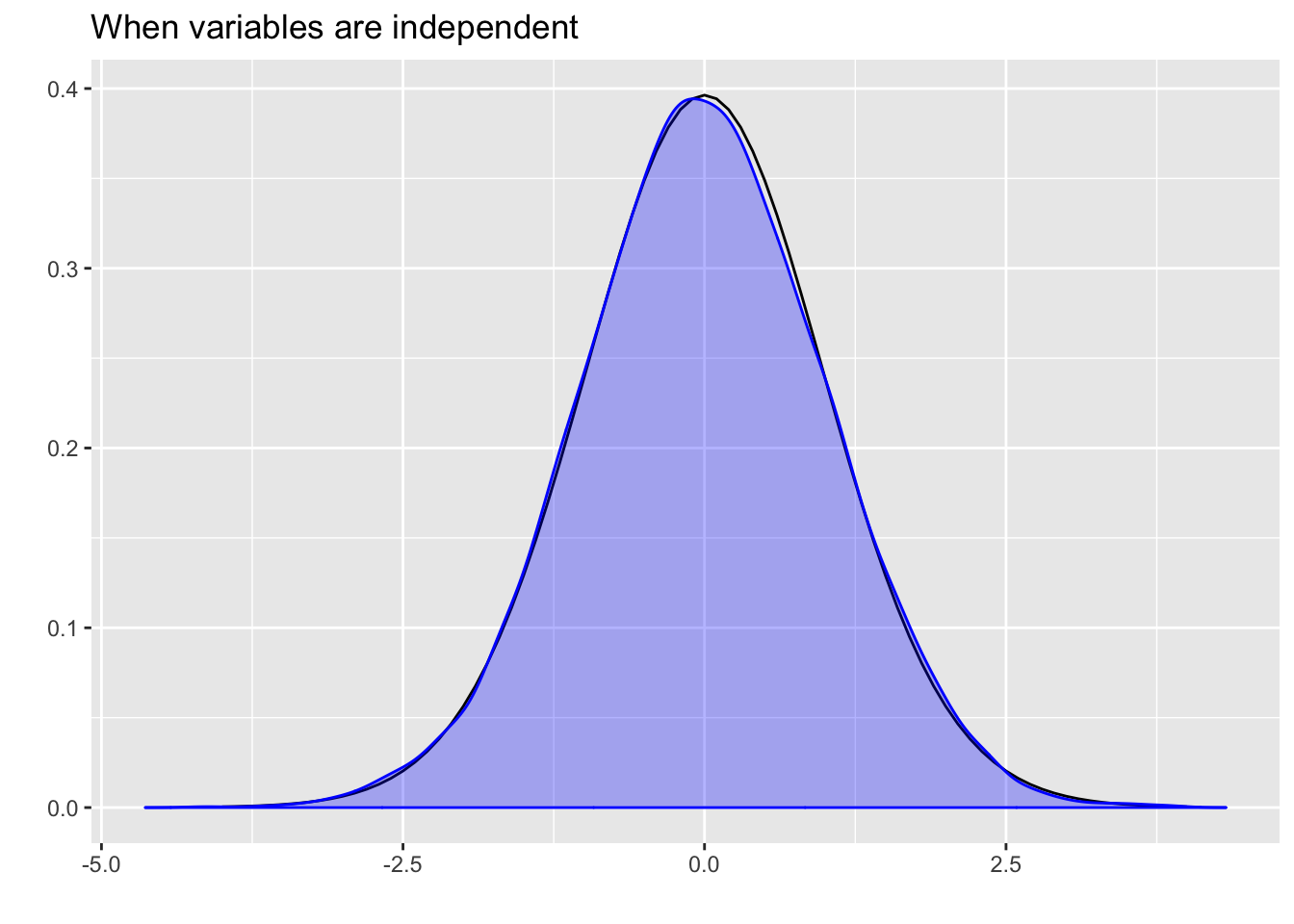
ts <- replicate(10000,rbvn_t(n=20, mu1=1, s1=4, mu2=1, s2=4, rho=0)$statistic)

Plotting the simulated samples shows that the empirical density curve nicely overlays the theoretical density for the t-distribution.

p <- ggdistribution(dt, df = 38, seq(-4, 4, 0.1)) 
autoplot(density(ts), colour = 'blue', p = p,  fill = 'blue') +
  ggtitle("When variables are independent")

Moreover, the 0.975 quantile, the value that would indicate the upper boundary for the acceptance region for an \(\alpha\) value of 0.05 is very close to the theoretical value of 2.024.

quantile(ts,.975)

## 97.5% 
## 1.996

qt(.975,38)

## [1] 2.024

Next, we simulate 10,000 small samples of 20 with a correlation of 0.3.

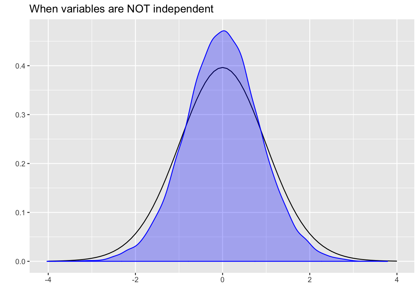
ts_d <- replicate(10000,rbvn_t(n=20, mu1=1, s1=4, mu2=1, s2=4, rho=.3)$statistic)

We see that now the fit is not so good. There simulated distribution has noticeably less probability in the tails.

pd <- ggdistribution(dt, df = 38, seq(-4, 4, 0.1)) 
autoplot(density(ts_d), colour = 'blue', p = pd,  fill = 'blue') +
  ggtitle("When variables are NOT independent")

The .975 quantile is much lower than the theoretical value of 2.024 showing that dependent data would lead to very misleading p-values.

quantile(ts_d,.975)

## 97.5% 
##  1.73

Summary

Properly performing a t-test on data obtained from an experiment could mean doing a whole lot of up front work to design the experiment in a way that will make the assumptions plausible. One could argue that the real practice of statistics begins even before making exploratory plots. Doing statistics with found data is much more problematic. At a minimum, doing a simple t-test means acquiring more that a superficial understanding of how the data were generated.

Finally, when all is said and done, and you have a well constructed t-test that results in a sufficiently small p-value to reject the null hypothesis, you will have attained what most people call a statistically significant result. However, I think this language misleadingly emphasizes the mechanical grinding of the “steel trap” logic of the test that I mentioned above. Maybe instead we should emphasize the work that went into checking assumptions, and think about hypothesis tests as producing “plausibly significant” results.

Some resources for doing t-tests in R

• Holmes and Huber (2019) Modern Statistics for Modern Biology, Chapter 6,

• Orloff and Bloom (2014) Null Hypothesis Significance Testing II

• Poldrack (2018) Statistical Thinking for the 21st century, Chapter 9

• Spector Using t-tests in R

• Wetherill (2015) How to Perform T-tests in R