Functional PCA with R

Definitions

• A Hilbert Space \(\mathscr{H}\) is an infinite dimensional vector space with an inner product denoted by \(<.,.>\). In our case, the vectors are functions.
• \(\mathscr{H}\) is separable if there exists an orthonormal basis. That is, there is an orthogonal collection of functions \((e_i)\) in \(\mathscr{H}\) such that \(<e_i,e_j>\; = 0\) if \(i = j\) and 0 otherwise, and every function in \(\mathscr{H}\) can be represented as a linear combination of these functions.
• The inner product of two functions \(X\) and \(Y\) in \(\mathscr{H}\) is defined as \(<X,Y>\; = \int X(\omega,t) Y(\omega,t)dt\).
• The norm of \(X\) is defined in terms of the inner product: \(\parallel X(\omega) \parallel ^2\; = \int X(\omega, t)^2 dt < \infty\).
• \(X\) is said to be square integrable if \(E\parallel X(\omega) \parallel ^2 < \infty\).
• The covariance operator \(C(y): \mathscr{H} \Rightarrow \mathscr{H}\) for any square integrable function \(X\) is given by: \(C(y) = E[<X - EX,y>(X - EX)]\)

The Road to Functional Principal Components

As we have seen, the fundamental idea of Functional Data Analysis is to represent a function \(X\) by a linear combination of basis elements. In the previous posts we showed how to accomplish this using a basis constructed from more or less arbitrarily selected B-spline vectors. But, is there a an empirical, some would say natural basis that can be estimated from the data? The answer is yes, and that is what FPCA is all about.

A good way to start is to look at the distance between a vector \(X\) and its projection down into the space spanned by some finite, p-dimensional basis \((u_k)\) which is expressed in the following equation,

\(D = E\parallel X - \sum_{k=1}^{p}<X, u_k>u_k\parallel^2\)             \((*)\)

This expands out to:

\(= E [< (X - \sum_{k=1}^{p}<X, u_k>u_k, X - \sum_{k=1}^{p}<X, u_k>u_k)>]\)

and with a little algebra this:

\(= E\parallel X \parallel^2 - \sum_{k=1}^{p}E<X, u_k>^2\)

It should be clear that we would want to find a basis that makes \(D\) as small as possible, and that minimizing \(D\) is equivalent to maximizing the term to be subtracted in the line above.

A little algebra shows that, \(E<X, u_k>^2 \;=\; <C(u_k),u_k>\) where \(C(u_k)\) is the covariance operator defined above.

Now, we are almost at our destination. There is a theorem (e.g. Theorem 11.4.1 in reference 1.) that says for any fixed number of basis elements p, the distance D above is minimized if \(u_j = v_j\) where the \(v_j\) are the eigenfunctions of \(C(y)\) with respect to the unit norm. From this it follows that \(E<X, v_j>^2 \;=\; <C(v_,),v_j>\; =\; <\lambda_j, v_j>\; =\; \lambda_j\).

Going back to equation \((*)\), we can expand \(X\) in terms of the basis \((v_j)\) so \(D = 0\) and we have what is called the Karhunen–Loève expansion: \(X = \mu + \sum_{j=1}^{\infty}\xi_jv_j\)

where:

• \(\mu = EX\)
  
• The deterministic basis functions \((v_j)\) are called the functional principal components
• The \((v_j)\) have unit norm and are unique up to their signs. (You can work with \(v_j\) or \(-v_j\).)
• The eigenvalues are such that: \(\lambda_1 > \lambda_2 > . . . \lambda_p\)
• The random variables \(\xi_j =\; <X - \mu,v_j>\) are called the scores.
• \(E\xi_j = 0\), \(E\xi_j^2 = \lambda_j\) and \(E|\xi_i\xi_j| = 0,\; if\; i\;\neq\;j\).

And finally, with one more line:
\(\sum_{j=1}^{\infty}\lambda_j \: = \: \sum_{j=1}^{\infty}E[<X,v_j>^2] = E\sum_{j=1}^{\infty}<X,v_j>^2 \; = \; E\parallel X \parallel^2 \; < \infty\)

we arrive at our destination, the variance decomposition: \(E\parallel X - \mu \parallel^2 \;= \;\sum_{j=1}^{\infty}\lambda_j\)

Let’s Calculate

Now that we have enough math to set the context, let’s calculate. We will use the same simulated Brownian motion data that we used in the previous posts, and also construct the same B-spline basis that we used before and save it in the fda object W.obj. I won’t repeat the code here.

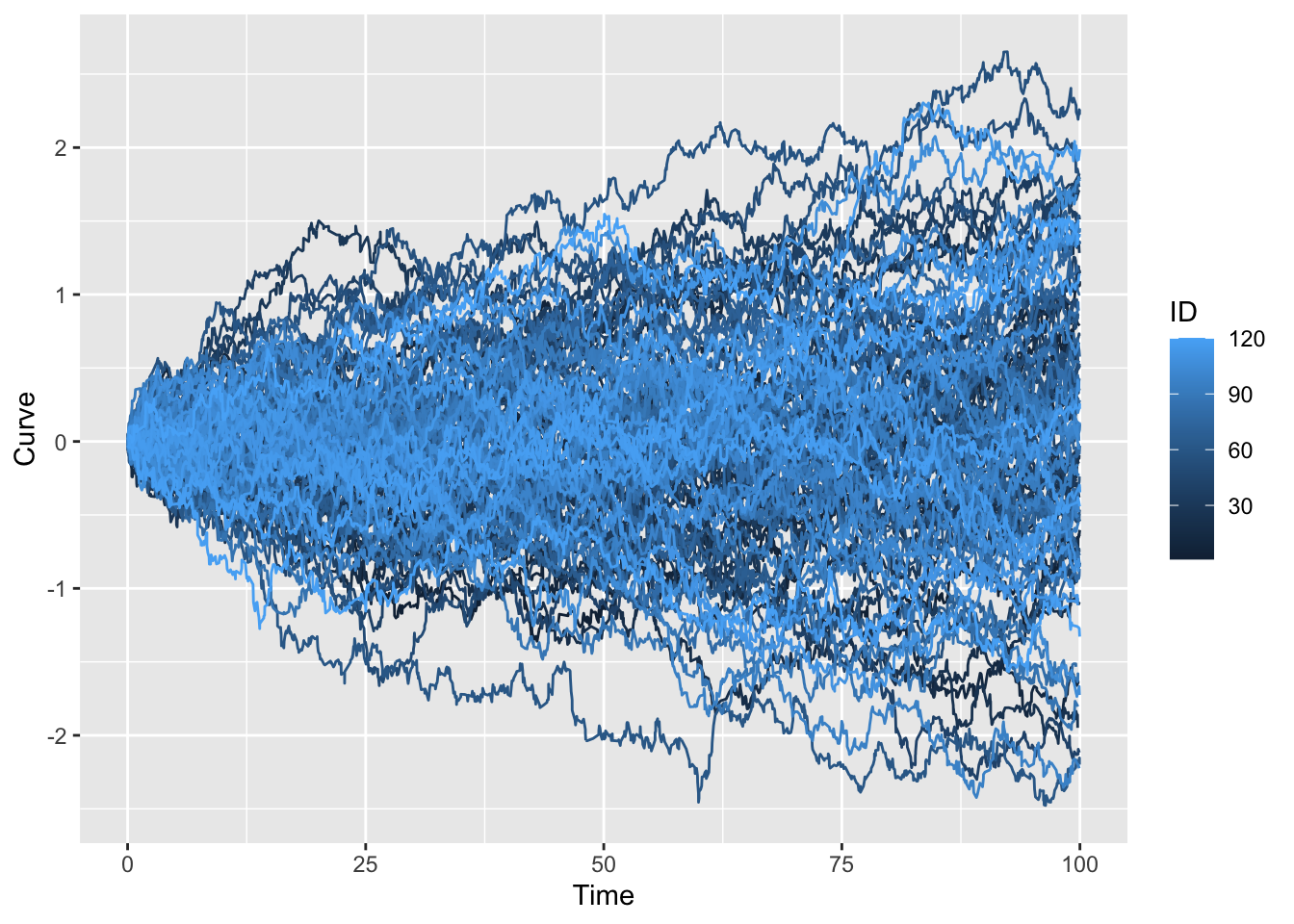
The following plot shows 120 simulated curves, each having 1000 points scattered over the interval [0, 100]. Each curve has unique observation times over that interval.

For first attempt at calculating functional principal components we’ll use the pca.fd() function from the fda package. So set up wise, we are picking up our calculations exactly where we left off in the previous post. As before, the basis representations of these curves are packed into the fda object W.obj. The function pca.fd() takes W.obj as input. It needs the non-orthogonal B-spline basis to seed its computations and the estimate the covariance matrix and the orthogonal eigenvector basis \(v_j\). The nharm = 5 parameter requests computing 5 eigenvalues.

The method of calculation roughly follows the theory outlined above. It starts with a basis representation of the functions, computes the covariance matrix, and calculates the eigenfunctions.

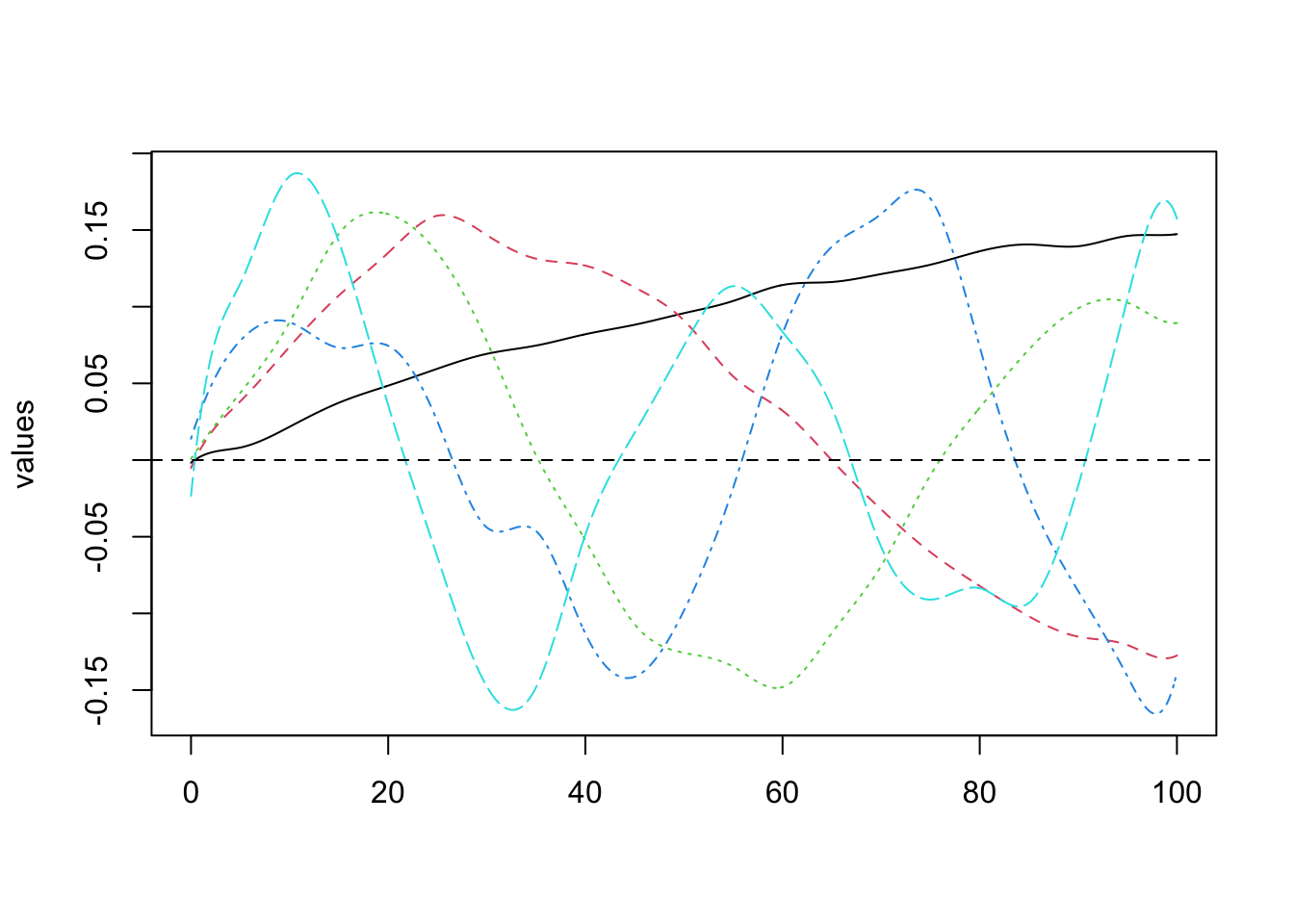
fun_pca <- pca.fd(W.obj, nharm = 5)

The object produced by pca.fd() is fairly complicated. For example, the list fun_pca$harmonics does not contain the eignevectors themselves, but rather coefficients that enable the eigenvectors to be computed from the original basis. However, because there is a special plot method for plot.pca.fd() it is easy to plot the eigenvectors.

plot(fun_pca$harmonics, lwd = 3)

## [1] "done"

It is also to obtain the eivenvalues \(\lambda_j\),

fun_pca$values

##  [1] 37.232207  3.724524  1.703604  0.763120  0.547976  0.389431  0.196101
##  [8]  0.163289  0.144052  0.116587  0.089307  0.057999  0.054246  0.050683
## [15]  0.042738  0.035107  0.031283  0.024905  0.019079  0.016428  0.011657
## [22]  0.007392  0.002664

and, the proportion of the variance explained by each eigenvalue.

fun_pca$varprop

## [1] 0.81965 0.08199 0.03750 0.01680 0.01206

A Different Approach

So far in this short series of FDA posts, I have been mostly using the fda package to calculate. In 2003 when it was released, it was ground breaking work. It is still the package that you are most likely to find when doing internet searches, and is the foundation for many subsequent R packages. However, as the CRAN Task View on Functional Data Analysis indicates, new work in FDA has resulted in several new R packages. The more recent fdapace takes a different approach to calculating principal components. The package takes its name from the (PACE) Principal Components by Conditional Expectation algorithm described in the paper by Yao, Müller and Wang (Reference 4. below). The package vignette is exemplary. It describes the methods of calculation, develops clear examples and provides a list of references to guide your reading about PACE and FDA in general.

A very notable feature of the PACE algorithm is that it is designed specifically to work with sparse data. The vignette describes the two different methods of calculation that package functions employ for sparse and non-sparse data. In this post, In this post we are not working with sparse data, but hope to do so in the future. See the vignette for examples of FPCA with sparse data.

library(fdapace)

The fdapace package requires data for the functions (curves) and associated times be organized in lists. We begin by using the fdapace::CheckData() function to check the data set up in the tibble df. (See previous post on descriptive statistics for the details on the data construction.)

CheckData(df$Curve,df$Time)

No error message is generated, so we move on th having the FPCA() function calculate the FPCA outputs including:

W_fpca <- FPCA(df$Curve,df$Time)

the eigenvalues:

W_fpca$lambda

## [1] 37.5386  3.2098  1.0210  0.3533

the cumulative percentage of variance explained by the eigenvalue

W_fpca$cumFVE

## [1] 0.8875 0.9634 0.9875 0.9959

and the scores:

head(W_fpca$xiEst)

##         [,1]    [,2]     [,3]     [,4]
## [1,]  0.8187  1.1971 -1.77755  0.20087
## [2,] -8.7396  2.4165 -0.33768 -0.10565
## [3,] -2.7517 -0.4879 -0.06747 -0.13953
## [4,]  3.9218  0.9419  0.39098 -0.25449
## [5,] -1.4400  0.7691  2.11549 -0.59947
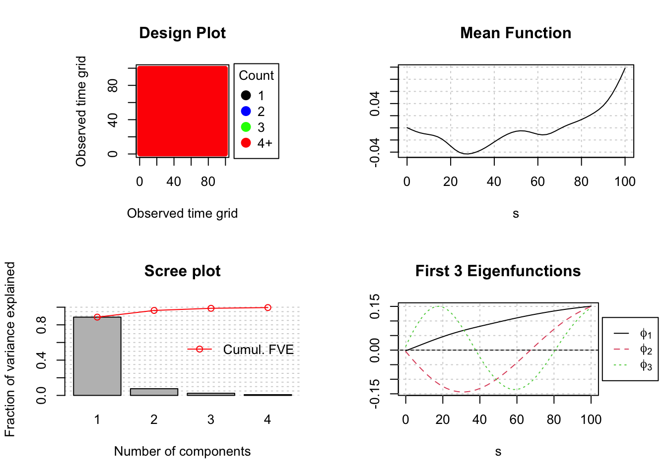
## [6,]  7.3952  0.5114 -2.16391  0.05199

All of these are in fairly good agreement with what we computed above. I am, however, a little surprised by the discrepancy in the value of the second eigenvalue. The default plot method for FPCA() produces a plot indicating the density of the data, a plot of the mean of the functions reconstructed from the eigenfunction expansion, a scree plot of the eigenvalues and a plot of the first three eigenfunctions.

plot(W_fpca)

Finally, it has probably already occurred to you that if you know the eigenvalues and scores, the Karhunen–Loève expansion can be used to simulate random functions. It can be shown that for the Wiener process:

\(v_j(t) = \sqrt2 sin(( j - \frac{1}{2})\pi t)\) and \(\lambda_j = \frac{1}{(j - \frac{1}{2})^2\pi^2}\)

This gives us:

\(W(t) = \sum_{j=1}^{\infty} \frac {\sqrt2}{(j - \frac{1}{2})\pi)} N_j sin(( j - \frac{1}{2})\pi t\)

where the \(N_j \:are\; iid \;N(0,1)\).

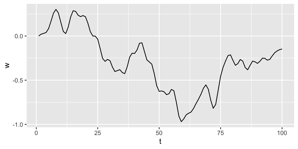
The fdapace function fdapace::Wiener() uses this information to simulate an alternative, smoothed version of the Brownian motion, Wiener process.

set.seed(123)
w <- Wiener(n = 1, pts = seq(0,1, length = 100))
t <- 1:100
df_w <- tibble(t, as.vector(w))
ggplot(df_w, aes(x = t, y = w)) + geom_line()

In future posts, I hope to continue exploring the fdapace package, including its ability to work with sparse data.

References

I found the following references particularly helpful.

1. Kokoszka, P. and Reimherr, M. (2017). Introduction to Functional Data Analysis. CRC.
2. Hsing, T and Eubank, R. (2015). Theoretical Foundations of Functional Data Analysis, with an Introduction to Linear Operators Wiley
3. Wang, J., Chiou, J. and Müller, H. (2015). Review of Functional Data Analysis
4. Yao, F., Müller, H, Wang, J. (2012). Functional Data Analysis for Sparse Longitudinal Data JASA J100, I 470