Intro

By now, I’m sure most people are familiar with the viral game Wordle. If you’ve been living under a rock and have no idea what I’m talking about, I recommend playing it for yourself. The best way I can describe it is: Take the classic board game Mastermind, but play with words instead of colored pegs. It’s a fun little game that encourages sharing and comparing scores with your friends – which I think explains a lot of its popularity!

Speaking of comparing scores, my wife routinely gets a better score than I do, so I’ve been trying to come up with better strategies. A few weeks ago, YouTube recommended 3Blue1Brown’s fantastic video on information theory and Wordle strategy. After watching it, I felt inspired. I could do something along those lines! Granted, I’m nowhere near as sophisticated as the creator of that video, but I thought it would be a fun challenge to crack open the game’s script and see what I could do with its data. With all the background out of the way, let’s jump into it!

Getting Started

First, we will need to include a number of libraries for this analysis. Most of these should be familiar to anyone who works with R regularly so I won’t add more color here.

suppressMessages({
library(httr)
library(dplyr)
library(stringr)
library(ggplot2)
library(ggthemes)
library(scales)
library(tidyr)})

From the 3B1B video, I found out you can view the code powering Wordle simply by viewing the page source in your browser and finding the JavaScript. As of writing, that code is here. Now, I’ll admit, I don’t know much of anything about JavaScript, but that doesn’t really matter – the word list is stored in plain text as an array.

If you look through the code, you might notice there are actually 2 word lists: The first, called Ma, is a list of 2,309 words that Wordle uses for puzzle solutions (there used to be 2,315 but apparently the NYT removed a few). The second list, called Oa, is a list of words it will accept as valid guesses. Since Oa has a lot more obscure words that will never show up as the answer, for this exercise, I am focusing entirely on Ma.

The first thing I do is simply download the .js file and save it as a giant string of text, which I’m calling wordle_script_text. In the event the script or domain name ever changes, all you need to do is paste in the new URL here.

url = "https://www.nytimes.com/games/wordle/main.18637ca1.js"
wordle_script_text = GET(url) %>%
  content(as = "text", encoding = "UTF-8")

Parsing the Word List

Next, I’m doing something messy that deserves some more explanation. I couldn’t figure out a good way to programmatically extract the entire word list by looking for the start and end points of the array, so instead, I scrolled through it in a text editor and manually identified the first and last words (cigar and shave, respectively). Then I told R to look for those particular words and extract everything between the two. It’s not ideal since rearranging the word list would completely break the rest of my script, so I’m open to any suggestions here!

Anyway, that left me with a giant string of comma separated words. From there, I removed any escaped quotation marks and separated each word into its own element by splitting the string at each comma. Then I converted all of that to a data frame where each row is a word, renamed the column, and converted every word to upper case. I call this data frame word_list.

word_list = substr(
  wordle_script_text,
  # cigar is the first word
  str_locate(wordle_script_text, "cigar")[,"start"],
  # shave is the last word
  str_locate(wordle_script_text, "shave")[,"end"]) %>%
  str_remove_all("\"") %>%
  str_split(",") %>%
  data.frame() %>%
  select(word = 1) %>%
  mutate(word = toupper(word))

Now we have our word list!

##    word
## 1 CIGAR
## 2 REBUT
## 3 SISSY
## 4 HUMPH
## 5 AWAKE

Determining Overall Letter Frequency

From there, my first idea was to get a frequency diagram of how often each letter appears. After all, intuitively, you wouldn’t expect letters like “X” to show up very often so it doesn’t make a lot of sense to play a word with “X” in it (unless you have a good reason). In the code below, I’m taking word_list and converting it back to a character vector, splitting every single character into its own element, and converting to a data frame again. I’m calling this data frame letter_list.

At this point, I should clarify why I did filter(row_number() != 1). R added a c() when I converted to a vector, which I don’t want to count towards the letter counts. This filter removes that extra c.

Continuing with the rest of the code, I renamed the column, filtered for upper-case letters only, and summarized by letter counts in descending order.

letter_list = word_list %>%
  as.character() %>%
  str_split("") %>%
  data.frame() %>%
  filter(row_number() != 1) %>%
  select(letter = 1) %>%
  filter(letter %in% LETTERS) %>%
  group_by(letter) %>%
  summarize(freq = n()) %>%
  arrange(desc(freq))

And now we have our frequency by letter!

## # A tibble: 5 × 2
##   letter  freq
##   <chr>  <int>
## 1 E       1230
## 2 A        975
## 3 R        897
## 4 O        753
## 5 T        729

But this isn’t very easy to read. Let’s throw it into a plot. A few callouts here:

• By default, ggplot sorts the x axis in alphabetical order. reorder forces ggplot to put the most frequent observations first.
• I used stat = "identity" since we already summarized letter_list in the previous section.
• I used expand = c(0,0) to make the bars stretch all the way to the axis.

ggplot(letter_list, aes(x = reorder(letter, (-freq)), y = freq)) +
  geom_bar(fill = "lightblue",
           stat = "identity") +
  geom_text(aes(x = reorder(letter, (-freq)),
                y = freq,
                label = comma(freq, accuracy = 1),
                vjust = 1),
            size = 2) +
  scale_y_continuous(labels = comma,
                     expand = c(0,0)) +
  theme_clean() +
  xlab("Letter") +
  ylab("Frequency") +
  labs(caption = "Generated by Arthur Holtz\nlinkedin.com/in/arthur-holtz/") +
  ggtitle("Letter Frequency in Wordle's Official Word List")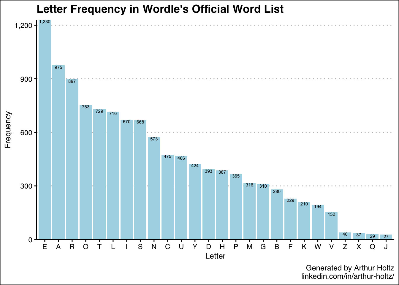

Much better! Looking at this plot, my naive strategy is to open with words containing letters on the left side of the plot. They’re much more likely to show up – but even if they don’t, knowing that is also valuable information. So maybe something like “TEARS” or “IRATE” (my wife’s favorite) is a good starter. One interesting thing to note is that this doesn’t match the overall letter frequency in English.

Determining Letter Frequency for Each Position

That’s all good to know, but I want more. Where do we go next? I got to thinking it would be helpful to know which letters are most likely to appear where.

To that end, I took word_list and split each letter into its own column. R added an empty column when I tried to do this, so I had to add an extra column (into = as.character(1:6)) and then remove the empty one and rename the others (the select). Ugh, whatever. I called this data frame ordered_letter_list.

ordered_letter_list = word_list %>%
  separate(word,
           sep = "",
           into = as.character(1:6)) %>%
  select(-1,
         "l_1" = 2,
         "l_2" = 3,
         "l_3" = 4,
         "l_4" = 5,
         "l_5" = 6)

Now we have a set of data that looks like this:

##   l_1 l_2 l_3 l_4 l_5
## 1   C   I   G   A   R
## 2   R   E   B   U   T
## 3   S   I   S   S   Y
## 4   H   U   M   P   H
## 5   A   W   A   K   E

I wanted to plot each of these letter positions on its own chart, so I first created a function called build_df that we can call in a for loop that only takes one column at a time and summarizes it with the most to least common letters.

build_df = function(df, col_name) {
  new_df = df %>%
    group_by(letter = eval(sym(col_name))) %>%
    summarize(freq = n()) %>%
    arrange(desc(freq))

  return(new_df)
}

Now we plug this function into a for loop to generate a plot for each letter position. Compared to the single plot before, there are some new things that are worth explaining:

• I create an object called letter_# and I set its value to be ordered_letter_list, but only including the letter number in question.
• Since we’re inside a for loop, ggplot won’t normally display plots. I wrap everything in print to make sure we can see the plots.

for (i in 1:5) {
  this_df = paste0("letter_", i)
  assign(this_df, build_df(ordered_letter_list, paste0("l_", i)))

  title = paste0("Letter # ", i, " Frequency in Wordle's Official Word List")

  print(ggplot(eval(sym(this_df)), aes(x = reorder(letter, (-freq)), y = freq)) +
    geom_bar(fill = "lightblue",
             stat = "identity") +
    geom_text(aes(x = reorder(letter, (-freq)),
                  y = freq,
                  label = comma(freq, accuracy = 1),
                  vjust = 1),
              size = 2) +
    scale_y_continuous(labels = comma,
                       expand = c(0,0)) +
    theme_clean() +
    xlab("Letter") +
    ylab("Frequency") +
    labs(caption = "Generated by Arthur Holtz\nlinkedin.com/in/arthur-holtz/") +
    ggtitle(title))
}

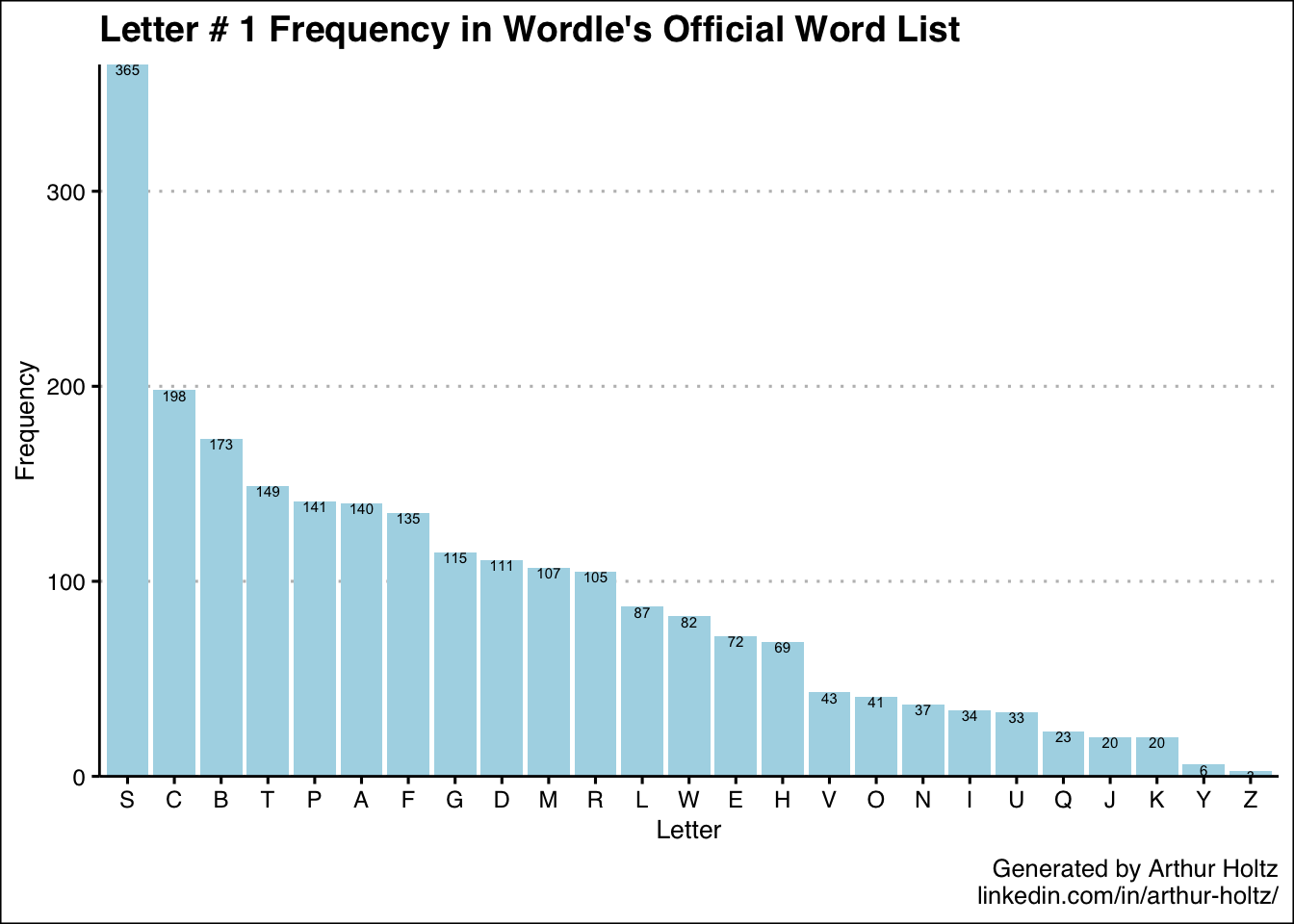
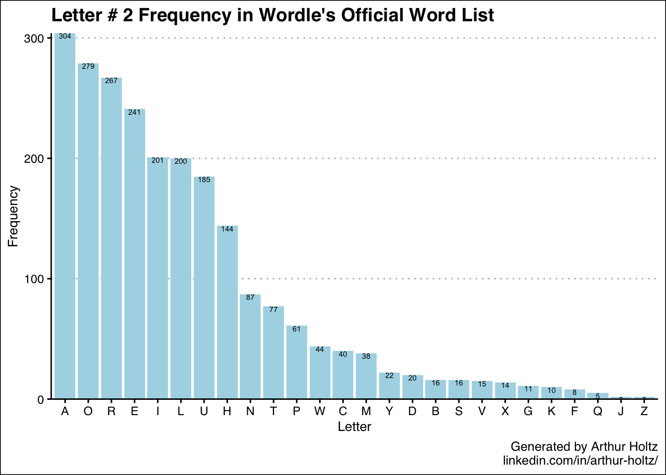
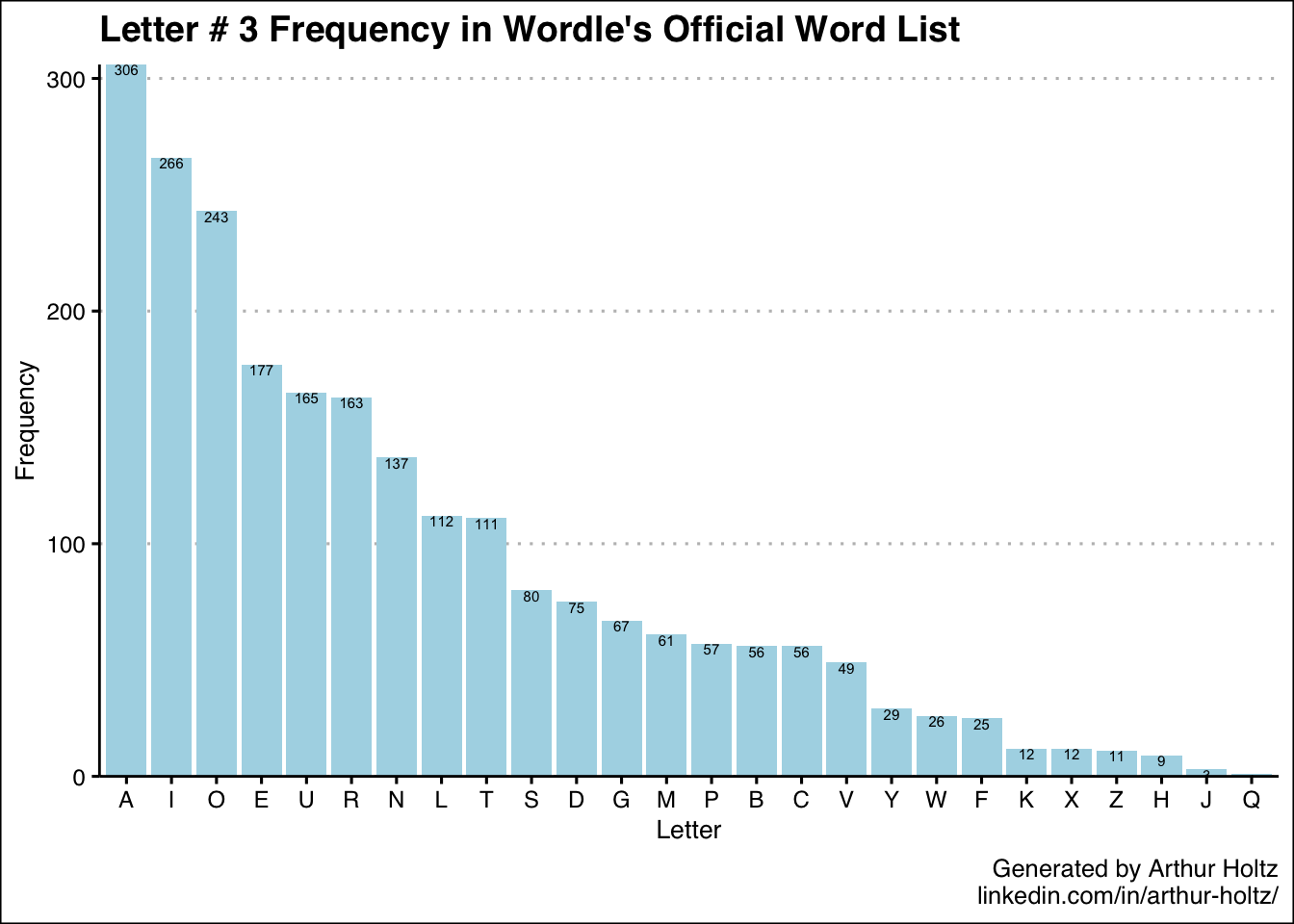
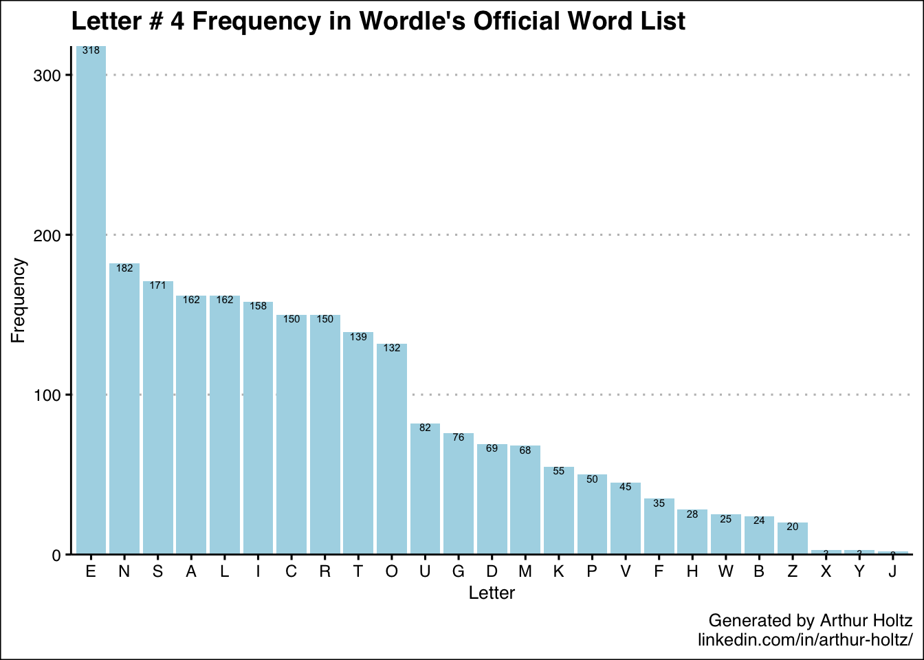
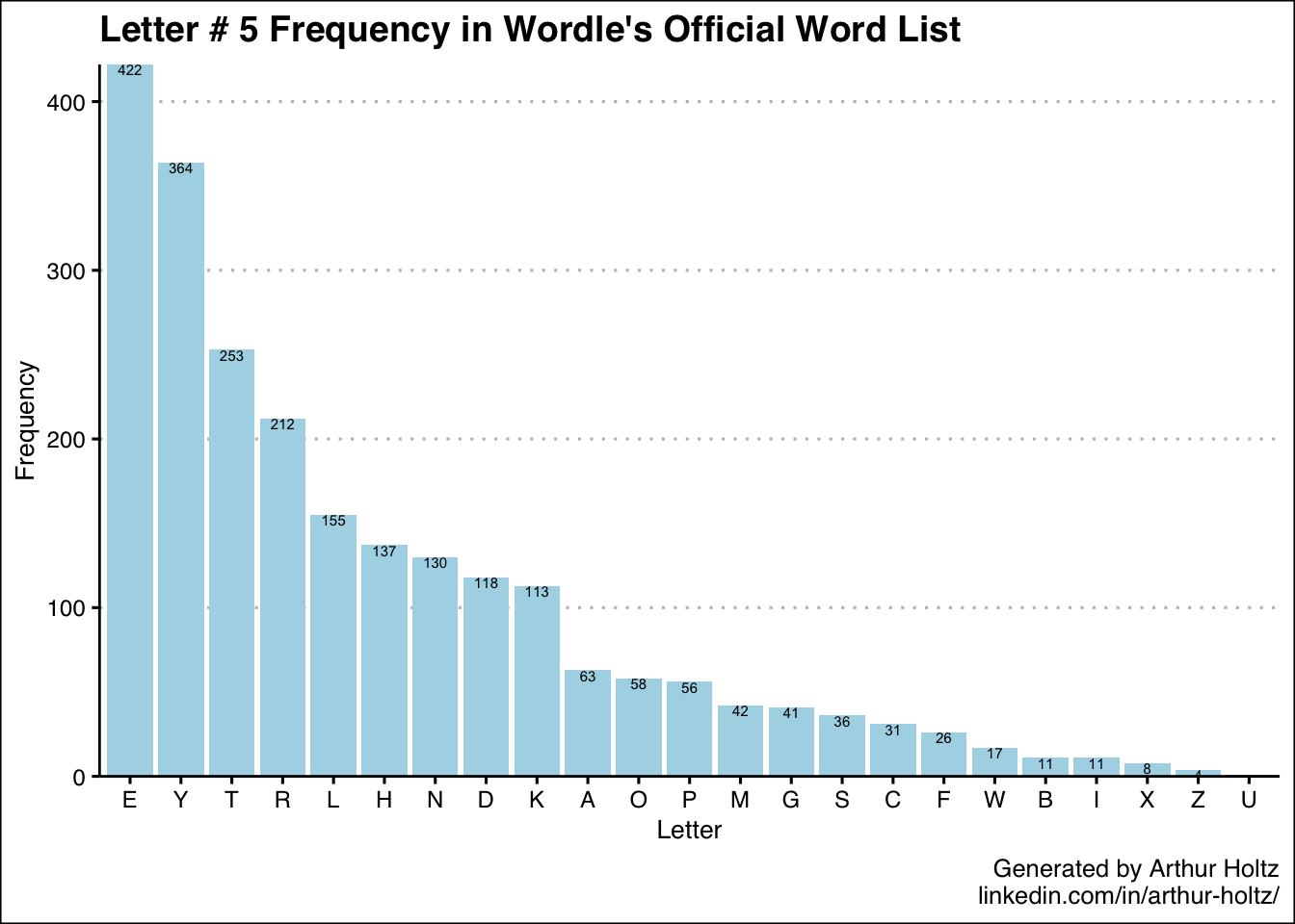With these 5 additional charts in my arsenal, now I know not only which letters are most common in general, but also where they are most likely to appear. One thing I was really surprised to find was just how uncommon “S” is as the 5th letter — only 36 out of 2,309 words! My best guess is the creators deliberately removed a number of plural words so there wouldn’t be so many words ending in “S.” It’s also neat how the 5 most frequent letters for the 3rd position are the vowels.

Brute Forcing Words with the Best “Score”

After discussing the initial analysis above with my dad, we came up with another idea: What if we took every word and bumped it up against every other word in Wordle’s list, and scored the guesses based on how much information they reveal on average?

I created a data frame called ordered_letter_list_rev that’s mostly the same as ordered_letter_list, except I only took the first 50 words (I’ll explain why later) and I kept the full word as the first column.

ordered_letter_list_rev = substr(
  wordle_script_text,
  str_locate(wordle_script_text, "cigar")[,"start"],
  str_locate(wordle_script_text, "shave")[,"end"]) %>%
  str_remove_all("\"") %>%
  str_split(",") %>%
  data.frame() %>%
  select(word = 1) %>%
  mutate(word = toupper(word)) %>%
  head(50) %>%
  separate(word,
           sep = "",
           into = as.character(1:6),
           remove = FALSE) %>%
  select(-2,
         "l_1" = 3,
         "l_2" = 4,
         "l_3" = 5,
         "l_4" = 6,
         "l_5" = 7)

Here is what it looks like:

##    word l_1 l_2 l_3 l_4 l_5
## 1 CIGAR   C   I   G   A   R
## 2 REBUT   R   E   B   U   T
## 3 SISSY   S   I   S   S   Y
## 4 HUMPH   H   U   M   P   H
## 5 AWAKE   A   W   A   K   E

Next, I created a data frame called cross_joined where I joined ordered_letter_list_rev to itself without any matching criteria. This is why I did head(50) in the previous section — the resulting data frame will square the row count of the original data frame, and I wanted to start with a reasonable-sized subset. If you have access to cloud computing resources, the sheer amount of data is less of a concern, but I’m running this on a personal computer, so bear with me.

Since this self-join would leave us with duplicate column names, I used suffixes = c("_guess","_target") in the merge function to distinguish the guesses from the target words. I also filtered out any rows where the guess is the same as the target since these cases don’t give us any useful information.

Next came the scoring. My (somewhat arbitrary) idea was to give 3 points for getting the right letter in the right place, 1 point for the right letter in the wrong place, and 0 points for wrong letters. I know I did this part extremely inefficiently since there’s a lot of copy/pasted code. I tried searching Stack Overflow for how to do this properly but eventually realized I had spent more time searching than I would have spent using good ol’ copy/paste in the first place. Again, if you know a better way, I’m wide open to suggestions!

cross_joined = merge(ordered_letter_list_rev,
                     ordered_letter_list_rev,
                     by = NULL,
                     suffixes = c("_guess","_target")) %>%
  filter(word_guess != word_target) %>%
  mutate(
    l_1_score = case_when(
      l_1_guess == l_1_target ~ 3,
      l_1_guess == l_2_target ~ 1,
      l_1_guess == l_3_target ~ 1,
      l_1_guess == l_4_target ~ 1,
      l_1_guess == l_5_target ~ 1,
      TRUE ~ 0),
    l_2_score = case_when(
      l_2_guess == l_2_target ~ 3,
      l_2_guess == l_1_target ~ 1,
      l_2_guess == l_3_target ~ 1,
      l_2_guess == l_4_target ~ 1,
      l_2_guess == l_5_target ~ 1,
      TRUE ~ 0),
    l_3_score = case_when(
      l_3_guess == l_3_target ~ 3,
      l_3_guess == l_1_target ~ 1,
      l_3_guess == l_2_target ~ 1,
      l_3_guess == l_4_target ~ 1,
      l_3_guess == l_5_target ~ 1,
      TRUE ~ 0),
    l_4_score = case_when(
      l_4_guess == l_4_target ~ 3,
      l_4_guess == l_1_target ~ 1,
      l_4_guess == l_2_target ~ 1,
      l_4_guess == l_3_target ~ 1,
      l_4_guess == l_5_target ~ 1,
      TRUE ~ 0),
    l_5_score = case_when(
      l_5_guess == l_5_target ~ 3,
      l_5_guess == l_1_target ~ 1,
      l_5_guess == l_2_target ~ 1,
      l_5_guess == l_3_target ~ 1,
      l_5_guess == l_4_target ~ 1,
      TRUE ~ 0),
    total_score = l_1_score + l_2_score + l_3_score + l_4_score + l_5_score) 

This gave me a data frame like this:

##   word_guess l_1_guess l_2_guess l_3_guess l_4_guess l_5_guess word_target
## 1      REBUT         R         E         B         U         T       CIGAR
## 2      SISSY         S         I         S         S         Y       CIGAR
## 3      HUMPH         H         U         M         P         H       CIGAR
## 4      AWAKE         A         W         A         K         E       CIGAR
## 5      BLUSH         B         L         U         S         H       CIGAR
##   l_1_target l_2_target l_3_target l_4_target l_5_target l_1_score l_2_score
## 1          C          I          G          A          R         1         0
## 2          C          I          G          A          R         0         3
## 3          C          I          G          A          R         0         0
## 4          C          I          G          A          R         1         0
## 5          C          I          G          A          R         0         0
##   l_3_score l_4_score l_5_score total_score
## 1         0         0         0           1
## 2         0         0         0           3
## 3         0         0         0           0
## 4         1         0         0           2
## 5         0         0         0           0

While exploring the data here, I noticed something strange. To illustrate, let’s take a look at the score breakdown for guessing MARRY when the target word is MAJOR.

##   l_1_score l_2_score l_3_score l_4_score l_5_score total_score
## 1         3         3         1         1         0           8

Notice letters 3 and 4 (both Rs) are getting 1 point each. That’s not right! There’s only one R in MAJOR so this guess should really only get 7 points. There were a number of other cases like this (ERASE was a major offender because it has 2 Es, which you might recall was the most common letter in Wordle overall). The scores for guesses like these are inflated, so I wouldn’t trust this scoring logic.

Conclusion

This is where I got stuck. It must be possible to only give points for repeat letters once if there is only one such letter in the answer — but how? I can’t figure it out without making a super-complicated case_when statement. If someone has a brilliant idea, I’d be thrilled to expand upon this analysis in a future update.

And where would you go next? Assuming I can solve the scoring problem, I’d also like to use the entire Oa word list as my guessing pool so I can find the most useful guesses, even if they won’t necessarily be the target word.

I hope you’ve enjoyed walking through Wordle’s code and word list with me! Even though I couldn’t complete all the analysis I originally set out to do, I’m just hoping the overall and by-location frequency analysis give me enough of an edge to do better than my wife!